clavibacter
16S Taxonomic exploration

In the last episode, We observed that the best database option to use is
Greengenes. With this in mind, I will do the analysis of the data that has
gone throught the 16-all-around.sh script.
I will use RStudio and mainly the package phyloseq to analyze the data.
Loadind the required packages
We will use the same amount of packages that we used on chapter 3:
> library("phyloseq")
> library("ggplot2")
> library("edgeR")
> library("DESeq2")
> library("RColorBrewer")
> library("stringr")
> library("sf")
> library("rnaturalearth")
> library("rnaturalearthdata")
> library("ggspatial")
> library("ggrepel")
> library("grid")
> library("gridExtra")
> library("ggmap")
> library("cowplot")
> library("ggsn")
> library("scatterpie")
> library("svglite")
> library("tidyverse")
Creatting a palette of colors
Since we will be using datasets from different host plants, it is convenient to create a pallete that will be used in all the plots:
> diverse.colors <- c("#1b9e77","#d95f02","#7570b3","#e7298a",
                    "#66a61e","#e6ab02","#a6761d","#666666")
Loading the biom files
As an output of the 16-all-around.sh program, we should have a biom file inside
each of the data folders. We will load them inside phyloseq objects:
> #Medicago sativa
> m.misce <- import_biom("medicago-sativa/miscellaneous/taxonomy/biom-files/medicago.biom")

> #Tuberosum
> t.misce <- import_biom("tuberosum/miscellaneous-tuberosum/taxonomy/biom-files/tuber.biom")
> t.shi <- import_biom("tuberosum/shi-2019/taxonomy/biom-files/tuber.biom")

> #Zea Mayz
> z.wu <- import_biom("zea-mayz/m-wu-2021/taxonomy/biom-files/zea.biom")
Now, I need to trim some of the information so as to be more meaningful:
> #Medicago sativa
> m.misce@tax_table@.Data <- substring(m.misce@tax_table@.Data, 4)
> colnames(m.misce@tax_table@.Data) <- c("Kingdom", "Phylum", "Class", "Order", "Family", "Genus", "Species")

> #Tuberosum
> t.misce@tax_table@.Data <- substring(t.misce@tax_table@.Data, 4)
> colnames(t.misce@tax_table@.Data) <- c("Kingdom", "Phylum", "Class", "Order", "Family", "Genus", "Species")
> t.shi@tax_table@.Data <- substring(t.shi@tax_table@.Data, 4)
> colnames(t.shi@tax_table@.Data) <- c("Kingdom", "Phylum", "Class", "Order", "Family", "Genus", "Species")
> #Zea Mayz
> z.wu@tax_table@.Data <- substring(z.wu@tax_table@.Data, 4)
> colnames(z.wu@tax_table@.Data) <- c("Kingdom", "Phylum", "Class", "Order", "Family", "Genus", "Species")
Loading and trimming the metadata
We will load each of the four metadata files from all our datasets:
> #Medicago sativa
> mraw.M.misce <- read.csv2(file = "medicago-sativa/miscellaneous/metadata/SraRunTable.txt", sep = ",")

> #Tuberosum
> mraw.T.misce <- read.csv2(file = "tuberosum/miscellaneous-tuberosum/metadata/SraRunTable.txt", sep = ",")
> mraw.T.misce <- mraw.T.misce[! mraw.T.misce$Run %in% c("SRR7881257","SRR7881260","SRR7881266","SRR7881267","SRR7881268",
                                                       "SRR7881270","SRR7881271","SRR7881272","SRR7881273"),]
> mraw.T.shi <- read.csv2(file = "tuberosum/shi-2019/metadata/SraRunTable.txt", sep = ",")

> #Zea Mayz
> mraw.Z.wu <- read.csv2(file = "zea-mayz/m-wu-2021/metadata/SraRunTable.txt", sep = ",")
> mraw.Z.wu <- mraw.Z.wu[(mraw.Z.wu$HOST == "Zea mays"),]
There are some actions that I want to talk about. In the tuberosum/miscellaneous-tuberosum/ dataset, the majority of the libraries were missing.
I need to erase them from the data table. I also need to obtain only the Zea mays
data from the zea-mays/m-wu-2021/, because this data is mixed with
Triticum information.
Trimming the metadata
As we explore the metadata , we will see that there is a lot of information. Some of that information we do not need it and some need to be trimmed to use it. We will stablish the same structure for each metadata. This will include the next fields (Columns in the data.frame):
- Sample: Name of the sample.
- Plant: The host-plant of the sample
- Environment: Environmental circunstances where the plant was sampled
- Isolation: Part of the plant where the microbiome was sampled
- State: Disease or Healthy, I will use the letters D and H.
- Latitude: Coordinates where the sample was taken.
- Longitude: Coordinates where the sample was taken.
> #Medicago sativa
> met.M.misce <- data.frame(row.names = mraw.M.misce$Run,
    	                      Plant = rep("Medicago",times = length(mraw.M.misce$Run)),
        	                  Sample = mraw.M.misce$Run,
            	              Environment = rep("Field",times = length(mraw.M.misce$Run)),
                	          Isolation = rep("Leave",times = length(mraw.M.misce$Run)),
            	              State = rep("Unknown",times = length(mraw.M.misce$Run)),
                    	      Latitude = as.numeric(c(37.24,37.23,37.22,37.21,37.20,
                            	                      37.19,37.18,37.17,37.16)),
                        	  Longitude = as.numeric(c(rep("115.1",times = length(mraw.M.misce$Run)/2),
                                        rep("113.52",times = length(mraw.M.misce$Run)/2))))
> #Tuberosum
> met.T.misce <- data.frame(row.names = mraw.T.misce$Run,
    	                      Plant = rep("Tuberosum",times = length(mraw.T.misce$Run)),
    	                      Sample = mraw.T.misce$Run,
        	                  Environment = rep("Field", times = length(mraw.T.misce$Run)),
            	              Isolation = rep("Rhizosphere", times = length(mraw.T.misce$Run)),
                	          State = rep("Unknown", times = length(mraw.T.misce$Run)),
                    	      Latitude = as.numeric(rep(32.03, times = length(mraw.T.misce$Run))),
                        	  Longitude = as.numeric(rep(118.46, times = length(mraw.T.misce$Run))) )

> met.T.shi <- data.frame(row.names = mraw.T.shi$Run,
	                        Plant = rep("Tuberosum",times = length(mraw.T.shi$Run)),
    	                    Sample = mraw.T.shi$Run,
        	                Environment = rep("Farm-Soil",times = length(mraw.T.shi$Run)),
            	            Isolation = c(rep("Soil",times = 19),rep("Rhizosphere",times = 20)),
                	        State = rep("D",times = length(mraw.T.shi$Run)),
                    	    Latitude =as.numeric(rep(34.2487,times = length(mraw.T.shi$Run))) ,
                        	Longitude =as.numeric(rep(119.8167,times = length(mraw.T.shi$Run))) )

#Zea Mayz
> met.Z.wu <- data.frame(row.names = mraw.Z.wu$Run,
	                       Plant = rep("Zea",times = length(mraw.Z.wu$Run)),
    	                   Sample = mraw.Z.wu$Run,
        	               Environment =rep("Field",times = length(mraw.Z.wu$Run)) ,
            	           Isolation = rep("Leave",times = length(mraw.Z.wu$Run)),
                	       State = rep("Unknown",times = length(mraw.Z.wu$Run)),
                    	   Latitude = as.numeric(substr(mraw.Z.wu$Lat_Lon, start = 0,stop = 5)) ,
                	       Longitude = as.numeric(substr(mraw.Z.wu$Lat_Lon, start = 9,stop = 14)))
Merging the information into new objects
First, we need to merge the phyloseq objects with its corresponding metadata
> #Medicago sativa
> m.misce <- merge_phyloseq(m.misce, sample_data(met.M.misce))

> #Tuberosum
> t.misce <- merge_phyloseq(t.misce, sample_data(met.T.misce))
> t.shi <- merge_phyloseq(t.shi, sample_data(met.T.shi))
> ##Merging the two individual object in one that contains all the Tuberosum data
> tuber <- merge_phyloseq(t.misce, t.shi)

> #Zea Mayz
> z.wu <- merge_phyloseq(z.wu, sample_data(met.Z.wu))
And bring all this information together into one phyloseq object and another
data.frame that will contain the metadata information from all the datasets:
> ##Merging all 4 complete objects in one
> bact.16S <- merge_phyloseq(m.misce,tuber,z.wu)
> ##Concentrating the metadata in one object
> all.meta<- rbind(met.M.misce, met.T.misce, met.T.shi, met.Z.wu)
Normalization of the data
If we explore the depth of the different data that we have, we will see that is different between every sample. Since we will begin to plot the data, we will define the a vector containing the colors assigned to each plant, thus we will have a constant color pattern for the plant factor in each of the plots:
> # We will create a vector to allocate the colors for each of the host plants that we have
> plant.colors <- diverse.colors[1:length(unique(all.meta$Plant))]
> names(plant.colors) <- unique(all.meta$Plant)

> #Allocating the taxonomic information into a data.frame
> dprof <- data.frame(Samples = as.factor(colnames(bact.16S@otu_table@.Data)),
  	                  Reads = sample_sums(bact.16S),
  	                  Plant = bact.16S@sam_data@.Data[[1]])
> #Ordering the factors to obtain the bars in order
> dprof$Samples <- factor(dprof$Samples, levels = dprof$Samples)

> #Plotting the obtained data
> ggplot(data = dprof, mapping = aes(x = Samples, y = Reads))+
  	geom_bar(stat = "identity", aes( fill = Plant)) +
  	scale_fill_manual(values = plant.colors)+
  	theme(text = element_text(size = 18),
    	    axis.text.x = element_text(angle = 90, hjust = 1, vjust = 0.5))+
  	geom_hline(yintercept = mean(sample_sums(bact.16S)), color = "cyan3",
    	         size = 1.5, alpha = 0.6)
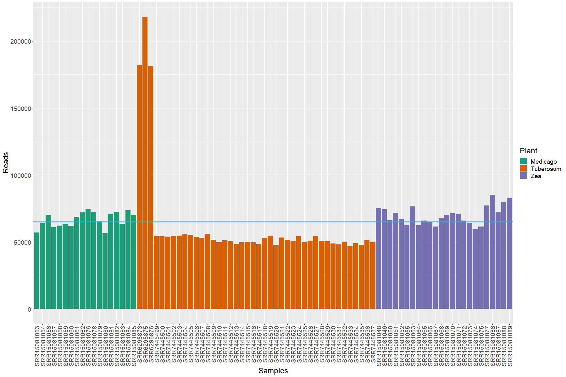
The cyan line marks the mean of the samples depth.
This makes is clear that the data needs normalization. McMurdi et al. found a great methodology to normalize the data. In their paper Waste Not, Want Not: Why Rarefying Microbiome Data Is Inadmissible they make an interesting discusion regarding this constant issue in this type of analysis. We will use their methodology:
> #-- Defining the normalization method --#
> edgeRnorm = function(physeq, ...) {
  	require("edgeR")
  	require("phyloseq")
  	# physeq = simlist[['55000_1e-04']] z0 = simlisttmm[['55000_1e-04']] physeq
  	# = simlist[['1000_0.2']] z0 = simlisttmm[['1000_0.2']] Enforce orientation.
  	if (!taxa_are_rows(physeq)) {
  	  physeq <- t(physeq)
  	}
  	x = as(otu_table(physeq), "matrix")
  	# See if adding a single observation, 1, everywhere (so not zeros) prevents
  	# errors without needing to borrow and modify calcNormFactors (and its
  	# dependent functions) It did. This fixed all problems.  Can the 1 be
  	# reduced to something smaller and still work?
  	x = x + 1
  	# Now turn into a DGEList
  	y = edgeR::DGEList(counts = x, remove.zeros = TRUE)
  	# Perform edgeR-encoded normalization, using the specified method (...)
  	z = edgeR::calcNormFactors(y, ...)
  	# A check that we didn't divide by zero inside `calcNormFactors`
  	if (!all(is.finite(z$samples$norm.factors))) {
  	  stop("Something wrong with edgeR::calcNormFactors on this data, non-finite $norm.factors")
  	}
  	# Don't need the following additional steps, which are also built-in to some
  	# of the downstream distance methods. z1 = estimateCommonDisp(z) z2 =
  	# estimateTagwiseDisp(z1)
  	return(z)
> }
> z<- edgeRnorm(bact.16S, method = "TMM")
> #-- Merging all the objects in the new normalized phyloseq object --#
> nor.cb <- merge_phyloseq(otu_table(z@.Data[[1]], taxa_are_rows = TRUE),
                         tax_table(bact.16S@tax_table@.Data),
                         bact.16S@sam_data)
> rm(z)
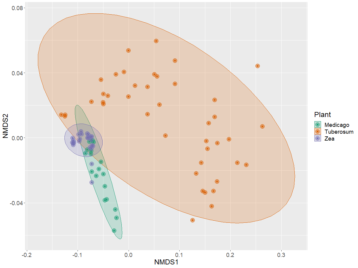
Analyzing the beta diversity
Now with this data, we can analyze how the taxonomic information of each sample is distributed across a NMDS ordination
> b16s.ord <- ordinate(physeq = nor.cb, method = "NMDS", distance = "bray")
> plot_ordination(physeq = nor.cb, ordination = b16s.ord,
  	              color = "Plant") +
  	stat_ellipse(geom = "polygon", alpha = 0.2, aes(fill = Plant))+
  	geom_point(size=5 , alpha = 0.5)+
  	scale_color_manual(values = plant.colors)+
  	scale_fill_manual(values = plant.colors)+
  	theme(text = element_text(size= 18))
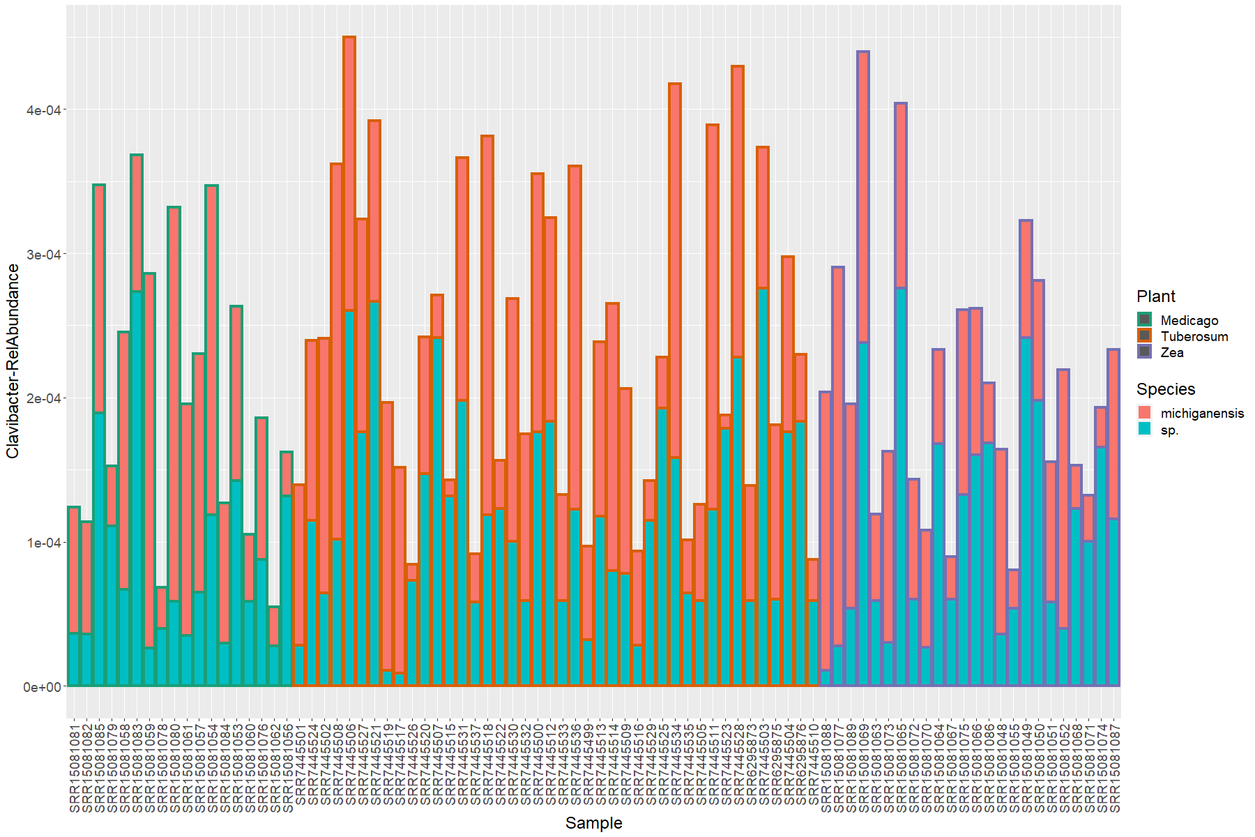
Obtaining and analyzing the Clavibacter data
With the next line of code we will obtain just the OTUs that were classified as Clavibacter as genus level:
> clabac <- subset_taxa(nor.cb, Genus == "Clavibacter")
Next, we will put this into a data.frame to plot the information. I will trim the species names of the Clavibacter that do not have a species assignation:
> clavi.df <- psmelt(clabac)
> clavi.df$Species[clavi.df$Species==""] <- "sp."
We will transform the data to relative abundance according to the total number of reads in each sample:
> clavi.df$ClaRelative <- sample_sums(clabac)/sample_sums(bact.16S)
Then, we will rearrenge the factor so as to gruop all the samples from the same plant host between each other:
> clavi.df$Sample <- as.factor(clavi.df$Sample)
> clavi.df <- arrange(.data = clavi.df, clavi.df$Plant)
> clavi.df$Sample <- factor(clavi.df$Sample, levels = unique(clavi.df$Sample))
Finally, let’s plot this data:
> ggplot(data = clavi.df, mapping = aes(y= ClaRelative, x = Sample, fill = Species, color = Plant))+
	  geom_bar(position = "stack", stat = "identity", size=1.5)+
	  scale_color_manual(values = plant.colors)+
	  ylab(label = "Clavibacter-RelAbundance")+
	  theme(text = element_text(size= 18),
    	    axis.text.x = element_text(angle = 90, hjust = 1, vjust = 0.5))