clavibacter
16S database exploration

kraken2 has the option to create databases of 16S using the information from three different repositories:
I will use the data obtained from Medicago sativa to explore if there are any substantial differences between the taxonomic assignation using each of the three databases.
Downloading the database
I prepared a folder named kraken with the next structure to download and index the 16S databases:
$ tree -L 2
.
└── database
    ├── datab03242022
    ├── gg04082022
    ├── rdp04082022
    └── silva04082022
Each of the three folders inside the database folder will contain a different
set of data. I named each database with the date it was created
since progess in bacterial taxonomic classification can bring substantial changes
in the future and an update will be needed.
I used the next piece of code to download the Greengenes, RPD, and
Silva databases:
$ kraken2-build --db gg04082022 --special greengenes --threads 12
$ kraken2-build --db rdp04082022 --special rdp --threads 12
$ kraken2-build --db silva04082022 --special silva --threads 12
The --threads flag can be customized to fulfill hardware requirements.
Downloading the reads from public databases (NCBI)
Let’s first downloaded them from the SRA repository in NCBI.
I will download the metadata table and the Accesion table. With the Accseion table I will use SRA-toolkit to download the 16S reads. I have created a
folder structure inside the clavibacter/16S main folder as follows:
$ tree -L 2
.
├── 16-S.Rproj
├── 16S-metadata
│   ├── m-wu-2021-SRR_Acc_List.txt
│   ├── m-wu-2021-SraRunTable.txt
│   ├── miscellaneous-SRR_Acc_List.txt
│   ├── miscellaneous-SraRunTable.txt
│   ├── miscellaneous-tuberosum-SRR_Acc_List.txt
│   ├── miscellaneous-tuberosum-SraRunTable.txt
│   ├── shi-2019-SRR_Acc_List.txt
│   └── shi-2019-SraRunTable.txt
├── medicago-sativa
│   ├── kraken-reads-v032822.sh
│   ├── kraken-reads-v042822.sh
│   ├── miscellaneous
│   ├── miscellaneous-SRR_Acc_List.txt
│   └── miscellaneous-SraRunTable.txt
├── tuberosum
│   ├── miscellaneous-tuberosum
│   ├── miscellaneous-tuberosum-SRR_Acc_List.txt
│   ├── miscellaneous-tuberosum-SraRunTable.txt
│   ├── shi-2019
│   ├── shi-2019-SRR_Acc_List.txt
│   └── shi-2019-SraRunTable.txt
└── zea-mayz
    ├── m-wu-2021
    ├── m-wu-2021-SRR_Acc_List.txt
    └── m-wu-2021-SraRunTable.txt
In this folder, I have downloaded and allocated all the metadata from the links
provided by my team. I will move to the medicago-sativa/miscellaneous subfolder
were I will download the data from the NCBI with the next command:
$ cat metadata/SRR_Acc_List.txt | while read line; do fasterq-dump $line -S -p -e 12; done
$ ls *.fastq | wc -l
36
Now, we have both the forward and reverse reads to begin to work with them. I am going to create a new folder to hoard the reads files and move the .fastq files
there. I will call this folder reads.
I want to use the information
inside the metadata table SraRunTable.txt to run the kraken commands, and also
to use it to run all the other programs that I will be using along this analysis.
Let’s see the structure of the file:
$ head -n 5 metadata/SraRunTable.txt
Run,Assay Type,AvgSpotLen,Bases,BioProject,BioSample,BioSampleModel,Bytes,Center Name,Collection_date,Consent,DATASTORE filetype,DATASTORE provider,DATASTORE region,env_broad_scale,env_local_scale,env_medium,Experiment,geo_loc_name_country,geo_loc_name_country_continent,geo_loc_name,HOST,Instrument,Lat_Lon,Library Name,LibraryLayout,LibrarySelection,LibrarySource,Organism,Platform,ReleaseDate,Sample Name,SRA Study
SRR15081053,WGS,494,29845998,PRJNA745034,SAMN20130882,"MIMS.me,MIGS/MIMS/MIMARKS.plant-associated",9181503,HEBEI UNIVERSITY,2019-08,public,"fastq,sra","gs,ncbi,s3","gs.US,ncbi.public,s3.us-east-1",plant,not collected,alfalfa,SRX11391104,China,Asia,"China:Hengshui City\,Hebei Province",Medicago sativa,Illumina MiSeq,37.24 N 115.10 E,ZTPSN19DC056,PAIRED,PCR,METAGENOMIC,metagenome,ILLUMINA,2021-07-09T00:00:00Z,G5_3,SRP327582
SRR15081054,WGS,495,33718905,PRJNA745034,SAMN20130881,"MIMS.me,MIGS/MIMS/MIMARKS.plant-associated",10544648,HEBEI UNIVERSITY,2019-08,public,"fastq,sra","gs,ncbi,s3","gs.US,ncbi.public,s3.us-east-1",plant,not collected,alfalfa,SRX11391103,China,Asia,"China:Hengshui City\,Hebei Province",Medicago sativa,Illumina MiSeq,37.23 N 115.10 E,ZTPSN19DC055,PAIRED,PCR,METAGENOMIC,metagenome,ILLUMINA,2021-07-09T00:00:00Z,G5_2,SRP327582
SRR15081056,WGS,492,36556092,PRJNA745034,SAMN20130880,"MIMS.me,MIGS/MIMS/MIMARKS.plant-associated",11372290,HEBEI UNIVERSITY,2019-08,public,"fastq,sra","gs,ncbi,s3","gs.US,ncbi.public,s3.us-east-1",plant,not collected,alfalfa,SRX11391101,China,Asia,"China:Hengshui City\,Hebei Province",Medicago sativa,Illumina MiSeq,37.22 N 115.10 E,ZTPSN19DC054,PAIRED,PCR,METAGENOMIC,metagenome,ILLUMINA,2021-07-09T00:00:00Z,G5_1,SRP327582
SRR15081057,WGS,493,33555059,PRJNA745034,SAMN20130879,"MIMS.me,MIGS/MIMS/MIMARKS.plant-associated",10652197,HEBEI UNIVERSITY,2019-08,public,"fastq,sra","gs,ncbi,s3","gs.US,ncbi.public,s3.us-east-1",plant,not collected,alfalfa,SRX11391100,China,Asia,"China:Hengshui City\,Hebei Province",Medicago sativa,Illumina MiSeq,37.21 N 115.10 E,ZTPSN19DC053,PAIRED,PCR,METAGENOMIC,metagenome,ILLUMINA,2021-07-09T00:00:00Z,G2_3,SRP327582
If I use the next piece of code, I can obtain the first column of all the rows, which is the Run information, the same name that each forward and reverse reads files has.
$ cat metadata/SraRunTable.txt| sed -n '1!p' | while read line; do read=$(echo $line | cut -d',' -f1); echo $read;done
SRR15081053
SRR15081054
SRR15081056
SRR15081057
SRR15081058
SRR15081059
SRR15081060
SRR15081061
SRR15081062
SRR15081076
SRR15081078
SRR15081079
SRR15081080
SRR15081081
SRR15081082
SRR15081083
SRR15081084
SRR15081085
This is going to be useful also to obtain all the other columns of information
inside the SraRunTable.txt file.
Taxonomic assignation with the three databases
In order to correctly annotate with the three different databases, I will create a
folder where I will save the output of each of the processes with kraken2. I will
create the greengenes, rdp, and silva folders to serve this purpose.
I prepared a little program that will obtain the needed information from each read
to run the kraken2 algorithm and to allocate the outputs in different folders,
this program is a variant of the all-around.sh that I have created along the
other episodes: 16-all-around.sh. This script can be locates on the scripts folder of this repository.
Let’s see what is inside:
$ cat 16-all-around.sh
#!/bin/sh
# This is a program that is going to pick a SraRunTable of metadata and
#extract the run label to run the next programs.

# This program requires that you give 3 input data. 1) where this
#SraRunTable is located, 2) where the kraken database has been saved,
# 3) a sufix that you want for the files to have (from the biom file, and to the extracted reads) and
# 4) The name of the author of the work

metd=$1 #Location to the SraRunTable.txt
kdat=$2 #Location of the kraken2 database
sufx=$3 #The choosen suffix for some files
aut=$4 #Author's name
root=$(pwd) #Gets the path to the directory of this file, on which the outputs ought to be created
# Now we will define were the reads are:
runs='reads'

# CREATING NECCESARY FOLDERS
mkdir reads
mkdir -p reads/clavi/
mkdir -p reads/cmm/
mkdir -p reads/fasta-clavi
mkdir -p taxonomy/kraken
mkdir -p taxonomy/taxonomy-logs/scripts
mkdir -p taxonomy/kraken/reports
mkdir -p taxonomy/kraken/krakens
mkdir -p taxonomy/biom-files


# DOWNLOADING THE DATA

#Let's use the next piece of code to download the data
cat $metd  |  sed -n '1!p' | while read line;  do read=$(echo $line | cut -d',' -f1); fasterq-dump -S $read -p -e 8 -o $read ; done
mv *.fastq reads/

# MANAGING THE DATA

# We will change the names of the reads files. They have a sufix that makes impossible
#to be read in a loop
ls $runs | while read line ; do new=$(echo $line | sed 's/_/-/g'); mv $runs/$line $runs/$new; done

# Now, we will create a file where the information of the run labes can be located
cat $metd  | while read line; do read=$(echo $line | cut -d',' -f1); echo $read ; done > run-labels.txt
mv run-labels.txt metadata/

# TAXONOMIC ASSIGNATION WITH KRAKEN2

cat metadata/run-labels.txt | while read line; do file1=$(echo $runs/$line-1.fastq); file2=$(echo $runs/$line-2.fastq) ; echo '\n''working in run' "$line"\
#kraken2 --db $kdat --threads 6 --paired $file1 $file2 --output taxonomy/kraken/krakens/$line.kraken --report taxonomy/kraken/reports/$line.report \
echo '#!/bin/sh''\n''\n'"kraken2 --db $kdat --threads 6 --paired" "$runs/$line"'-1.fastq' "$runs/$line"'-2.fastq' "--output taxonomy/kraken/krakens/$line.kraken --report taxonomy/kraken/reports/$line.report" > taxonomy/taxonomy-logs/scripts/$line-kraken.sh; sh taxonomy/taxonomy-logs/scripts/$line-kraken.sh; done

#CREATING THE BIOM FILE

# Now we will create the biom file using kraken-biom
kraken-biom taxonomy/kraken/reports/* --fmt json -o taxonomy/biom-files/$sufx.biom

# EXTRACTING THE CLAVIBACTER READS

# With the next piece of code, the reads clasiffied as from the genus "Clavibacter", will be separated from the main reads.
# The number needed for the extraction is the numeric-ID given to Clavibacter by kraken2: 1573
#EXTRACT THE READS IN FASTQ FORMAT
cat metadata/run-labels.txt | while read line;
do echo "\nExtracting Clavibacter reads in fastq from sample:" $line;
extract_kraken_reads.py -k taxonomy/kraken/krakens/$line.kraken -r taxonomy/kraken/reports/$line.report -s1 reads/$line-1.fastq -s2 reads/$line-2.fastq -o reads/clavi/$sufx-$aut-$line-clav-1.fq -o2 reads/clavi/$sufx-$aut-$line-clav-2.fq -t 1573 --fastq-output --include-children; done

#EXTRACT THE READS IN FASTA FORMAT
cat metadata/run-labels.txt | while read line;
do echo "\nExtracting Clavibacter reads in fasta from sample:" $line;
extract_kraken_reads.py -k taxonomy/kraken/krakens/$line.kraken -r taxonomy/kraken/reports/$line.report -s1 reads/$line-1.fastq -s2 reads/$line-2.fastq -o reads/fasta-clavi/$sufx-$aut-$line-clav-1.fasta -o2 reads/fasta-clavi/$sufx-$aut-$line-clav-2.fasta -t 1573 --include-children; done

# EXTRACTING THE CLAVIBACTER MICHIGANESIS-MICHIGANENSIS READS

# With the next piece of code, the reads clasiffied as from the Clavibacter michiganensis michiganensis, will be separated from the main reads.
# The number needed for the extraction is the numeric-ID given to Cmm by kraken2: 33013

cat metadata/run-labels.txt | while read line;
do echo "\nExtracting Cmm reads in fasta format from sample:" $line; extract_kraken_reads.py -k taxonomy/kraken/krakens/$line.kraken -r taxonomy/kraken/reports/$line.report -s1 reads/$line-1.fastq -s2 reads/$line-2.fastq -o reads/cmm/cmm-$sufx-$aut-$line-1.fq -o2 reads/cmm/cmm-$sufx-$aut-$line-2.fq -t 33013 --include-children; done
You can always change the number of threads to be used.
So, in my case I am going to run it with the following command to run kraken2 with
the Greengenes database:
$ sh kraken-all.sh metadata/SraRunTable.txt /mnt/d/programs/kraken/database/gg04082022 medicago misce
working in run SRR15081053
Loading database information... done.
60417 sequences (29.85 Mbp) processed in 2.690s (1347.6 Kseq/m, 665.72 Mbp/m).
  60400 sequences classified (99.97%)
  17 sequences unclassified (0.03%)

working in run SRR15081054
Loading database information... done.
68119 sequences (33.72 Mbp) processed in 3.005s (1360.0 Kseq/m, 673.20 Mbp/m).
  68019 sequences classified (99.85%)
  100 sequences unclassified (0.15%)
The resulting output is telling us that kraken2 is running on the files that
we gave to the program. It will take a several minutes to process this set of 18 samples.
In the end, we will have new content inside our new taxonomy folder:
$ tree -L 2
.
├── kraken
│   ├── biom-files
│   ├── krakens
│   └── reports
└── taxonomy-logs
    └── scripts
Inside the reports subfolder we can find all the resulting kraken-reports. I am
going to copy the information inside taxonomy to the greengenes folder to
continue with the new database and not re-write the information.
After running this code a third time with the Silva database, I have all the required information.
Taxonomic analysis in R
Using kraken-tools to create biom files
kraken-biom is a useful program that
can take different kraken-reports to assemble a biom file. I am going to create
a biom file inside each of the databases folders to begin wiht the analysis. The
next line of code can be used to create the one inside the greengenes folder:
$ kraken-biom kraken/reports/* -o ../bioms/greengenes.biom --fmt json
$ ls ../bioms/*.biom
greengenes.biom
I will do the same for the rest.
A broad comparison of the 3 databases
For the next section I will use RSutido to analize the taxonomic classification made by the three databases. I will use the next set of packages for this and future analyses on R:
| Package | Version | Link |
|---|---|---|
| Phyloseq | 1.36.0 | Page |
| ggplot2 | 3.3.5 | Page |
| edgeR | 3.34.1 | Page |
| DESeq2 | 1.32.0 | Page |
| pheatmap | 1.0.12 | Page |
| RColorBrewer | 1.1.2 | Page |
First of all, I load this package into my RStudio environmnet:
> library("phyloseq")
> library("ggplot2")
> library("edgeR")
> library("DESeq2")
> library("pheatmap")
> library("RColorBrewer")
I will use the function import_biom to load the biom files that I created .
First I will do this with the Silva results and prune the data.
> silva <- import_biom("medicago-sativa/miscellaneous/bioms/silva.biom")
> silva@tax_table@.Data <- substring(silva@tax_table@.Data, 4)
> colnames(silva@tax_table@.Data) <- c("Kingdom", "Phylum", "Class", "Order", "Family", "Genus", "Species")
I will do the same for the RPD and Greengenes data:
> ## The object obtained by pdp
> rdp <- import_biom("medicago-sativa/miscellaneous/bioms/rdp.biom")
> # Prunning the data
> rdp@tax_table@.Data <- substring(rdp@tax_table@.Data, 4)
> colnames(rdp@tax_table@.Data) <- c("Kingdom", "Phylum", "Class", "Order", "Family", "Genus", "Species")

> ## The object obtained by greengenes
> greeng <- import_biom("medicago-sativa/miscellaneous/bioms/greengenes.biom")
> # Prunning the data
> greeng@tax_table@.Data <- substring(greeng@tax_table@.Data, 4)
> colnames(greeng@tax_table@.Data) <- c("Kingdom", "Phylum", "Class", "Order", "Family", "Genus", "Species")
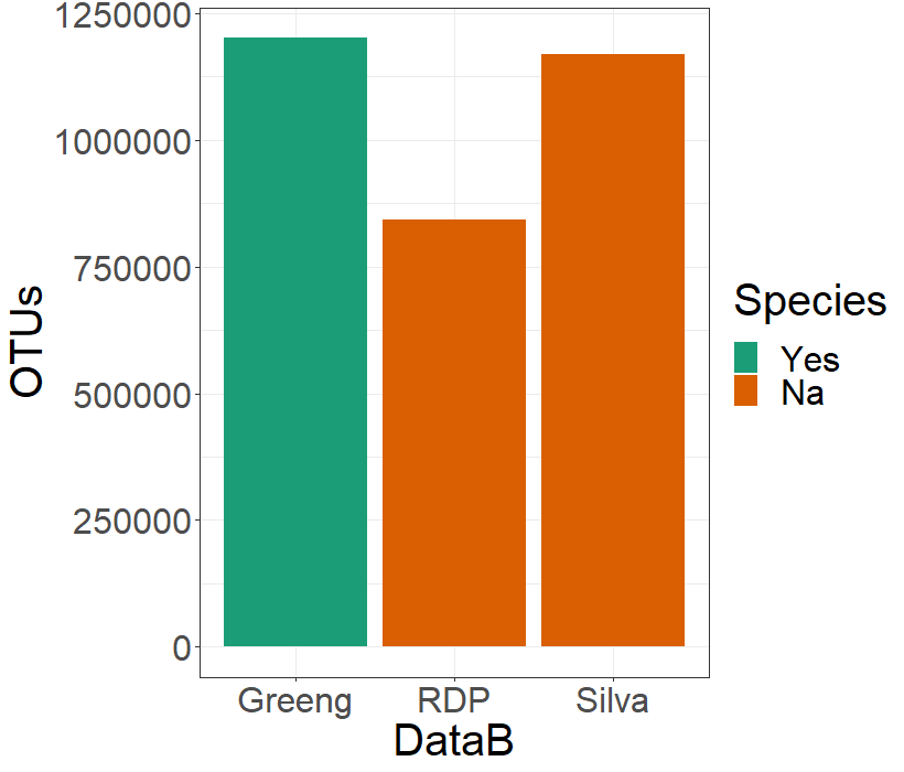
With this three objects on the phyloseq format, I will create a dataframe to allocate some metadata concerning the name of the database, the number of OTUS detected, how many non-bacterial OTUS the database detected, the number of unique Phyla found, and if the clasiffication with that database allowed the species identification of the OTUS:
> c.datab <- data.frame(row.names = c("Silva","RDP","Greeng"),
                      DataB = c("Silva","RDP","Greeng"),
                      OTUs = c(sum(sample_sums(silva)),sum(sample_sums(rdp)),
                               sum(sample_sums(greeng))),
                      NonBacteria = c(summary(silva@tax_table@.Data[,1] == "Bacteria")[2],
                                      summary(rdp@tax_table@.Data[,1] == "Bacteria")[2],
                                      summary(greeng@tax_table@.Data[,1] == "Bacteria")[2]),
                      Phyla = c(summary(unique(silva@tax_table@.Data[,2]))[1],
                                  summary(unique(rdp@tax_table@.Data[,2]))[1],
                                  summary(unique(greeng@tax_table@.Data[,2]))[1]),
                      Species= c("Na","Na","Yes"))
> c-datab
        DataB    OTUs NonBacteria Phylums Species
Silva   Silva 1168242          82      59      Na
RDP       RDP  842365           6      42      Na
Greeng Greeng 1200912           9      36     Yes
To look at this data in a graphical way, I will generate a plot. First I will choose which color I want to use with the next two lines:
> spe.color <- palette.colors(n = 2, palette = "Dark2")
> names(spe.color)<- c("Yes","Na")
And use the next code to create a bar-plot:
> ggplot(data = c.datab, aes(y = OTUs, x = DataB, fill = Species))+
    geom_bar(stat="identity", position=position_dodge())+
    scale_fill_manual(values = spe.color)+
    theme_bw() + theme(text = element_text(size = 20))
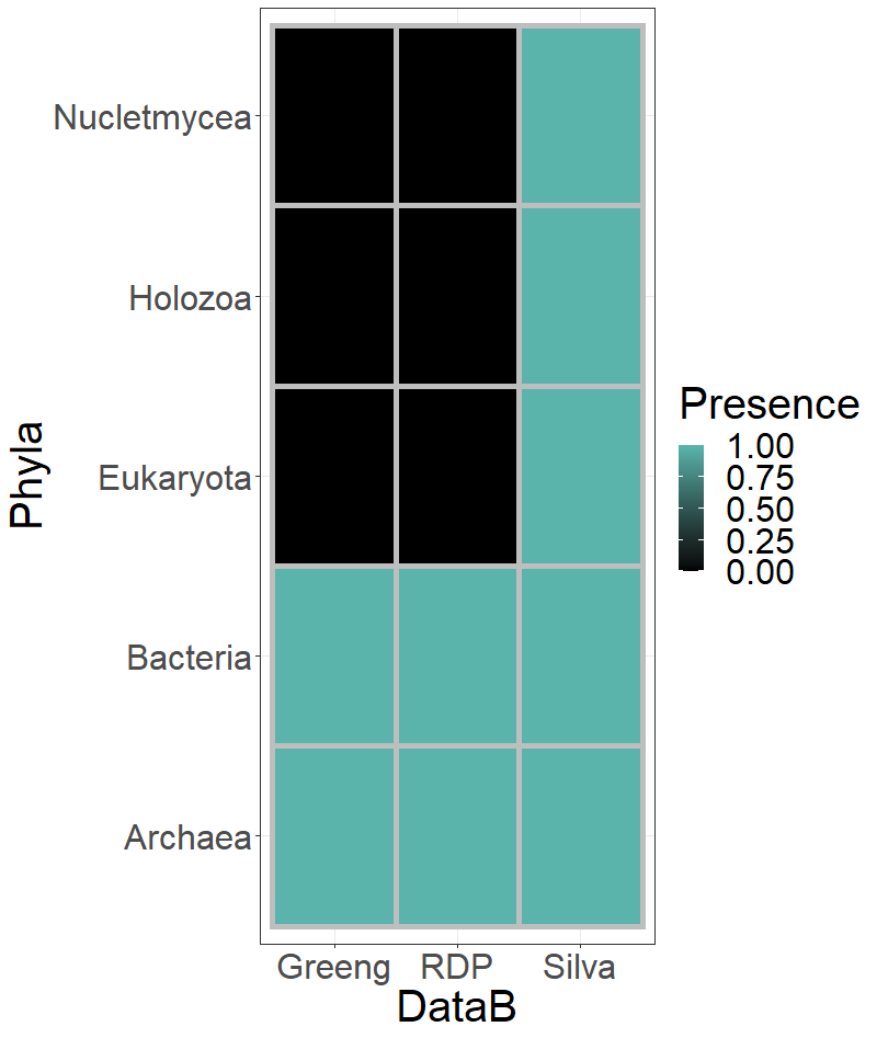
The number of reads deceted is important, but it is also important which OTUs can be detected with each of the databases. I am going to see which Phyla are being detected by each of the three databases. I am going to generate a dataframe to allocate this information:
> unique(greeng@tax_table@.Data[,1])
[1] "Bacteria" "Archaea"
> unique(rdp@tax_table@.Data[,1])
[1] "Bacteria" "Archaea"
> unique(silva@tax_table@.Data[,1])
[1] "Bacteria" "Holozoa" "Eukaryota" "Nucletmycea" "Archaea"
> heat.fra <- data.frame(DataB = c(rep(x = "Silva", times = 5),rep(x = "RDP", times = 5),
                                 rep(x = "Greeng", times = 5)),
                       Phyla = rep(x = unique(silva@tax_table@.Data[,1]), times = 3),
                       Presence = c(1,1,1,1,1,
                                    1,0,0,0,1,
                                    1,0,0,0,1))
With this information, I will use again ggplot2 to create a plot to show this
information.
> ggplot(data = heat.fra, mapping = aes(y= Phyla, x = DataB)) +
    geom_tile(aes(fill = Presence), colour = "grey", size = 2) +
    scale_fill_gradient(high = "#5ab4ac" ,low = "#000000" )+
    theme_bw() + theme(text = element_text(size = 30))
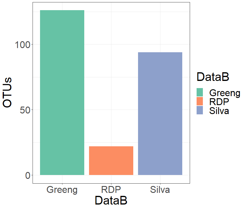
I would like to see how much Clavibacter reads were identified by each database. I will extract the Clavibacter data from all the phyloseq objects and trim the blanck space on Greengenes were no Species were identified:
> cla.silva <- subset_taxa(silva, Genus == "Clavibacter")
> cla.rdp <- subset_taxa(rdp, Genus == "Clavibacter")
> cla.greeng <- subset_taxa(greeng, Genus == "Clavibacter")
> cla.greeng@tax_table@.Data[1,7] <- "NotIdentified"
And I will use this information to draw a new bar-plot:
> #Dataframe of the Clavibacter OTUs
> clavi <- data.frame(DataB = c("Silva","RDP","Greeng"),
                    OTUs = c(sum(sample_sums(cla.silva)),sum(sample_sums(cla.rdp)),
                             sum(sample_sums(cla.greeng))))
> # Plotting
> ggplot(data = clavi, aes(y = OTUs, x = DataB, fill= DataB))+
    geom_bar(stat="identity", position=position_dodge())+
    scale_fill_brewer(type = "",palette = "Set2", aesthetics = "fill")+
    theme_bw() + theme(text = element_text(size = 30))
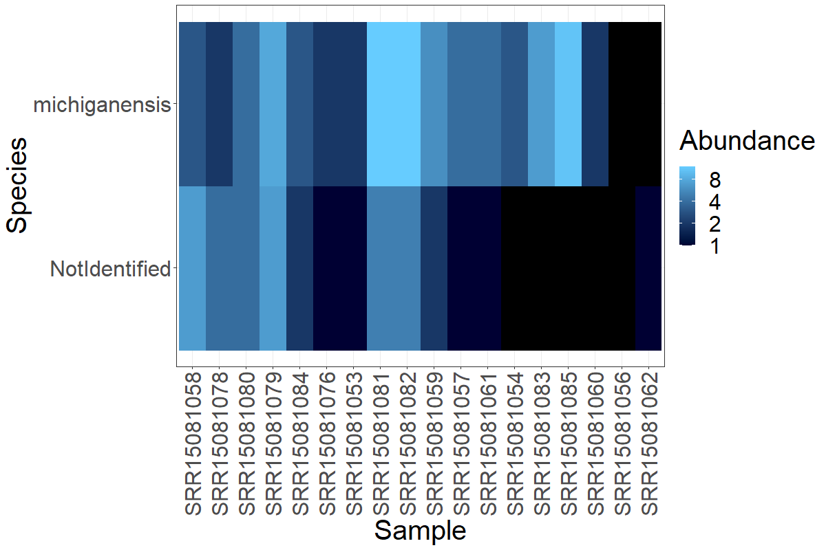
Finally, I would like to see how the Clavibacter OTUs are distributed on the Greengenes results, since this database was able to reach the Species level.
> plot_heatmap(cla.greeng, taxa.label = "Species") +
    theme_bw() + theme(text = element_text(size = 30))+
    theme(axis.text.x = element_text(angle = 90, vjust = 0.5, hjust=1))
Using Graphlan to create plots to compare the taxonomic assignation
I have wrote a markdown explaining the process to use the kraken outputs to plot
a dendogram using graphlan. I will use that knowledge to plot what I obtained
from the three different databases. To do an example, I am going to use the results
from Silva.
Inside the silva/ folder I created a new folder called grap/ where all the
data generated will be located. There, I will use the next line to create mpa
files:
$ mkdir mpa-files
$ ls ../kraken/reports/ | while read line; do name=$(echo $line | cut -d'.' -f1); kreport2mpa.py -r ../kraken/reports/$line -o mpa-files/$name.mpa; done
$ ls mpa-files/
SRR15081053.mpa  SRR15081058.mpa  SRR15081062.mpa  SRR15081080.mpa  SRR15081084.mpa
SRR15081054.mpa  SRR15081059.mpa  SRR15081076.mpa  SRR15081081.mpa  SRR15081085.mpa
SRR15081056.mpa  SRR15081060.mpa  SRR15081078.mpa  SRR15081082.mpa
SRR15081057.mpa  SRR15081061.mpa  SRR15081079.mpa  SRR15081083.mpa
With this information, I will combine all into a big file called combine.mpa
$ combine_mpa.py --input mpa-files/*.mpa --output mpa-files/combine.mpa
 Number of files to parse: 18
 Number of classifications to write: 2762
        2762 classifications printed
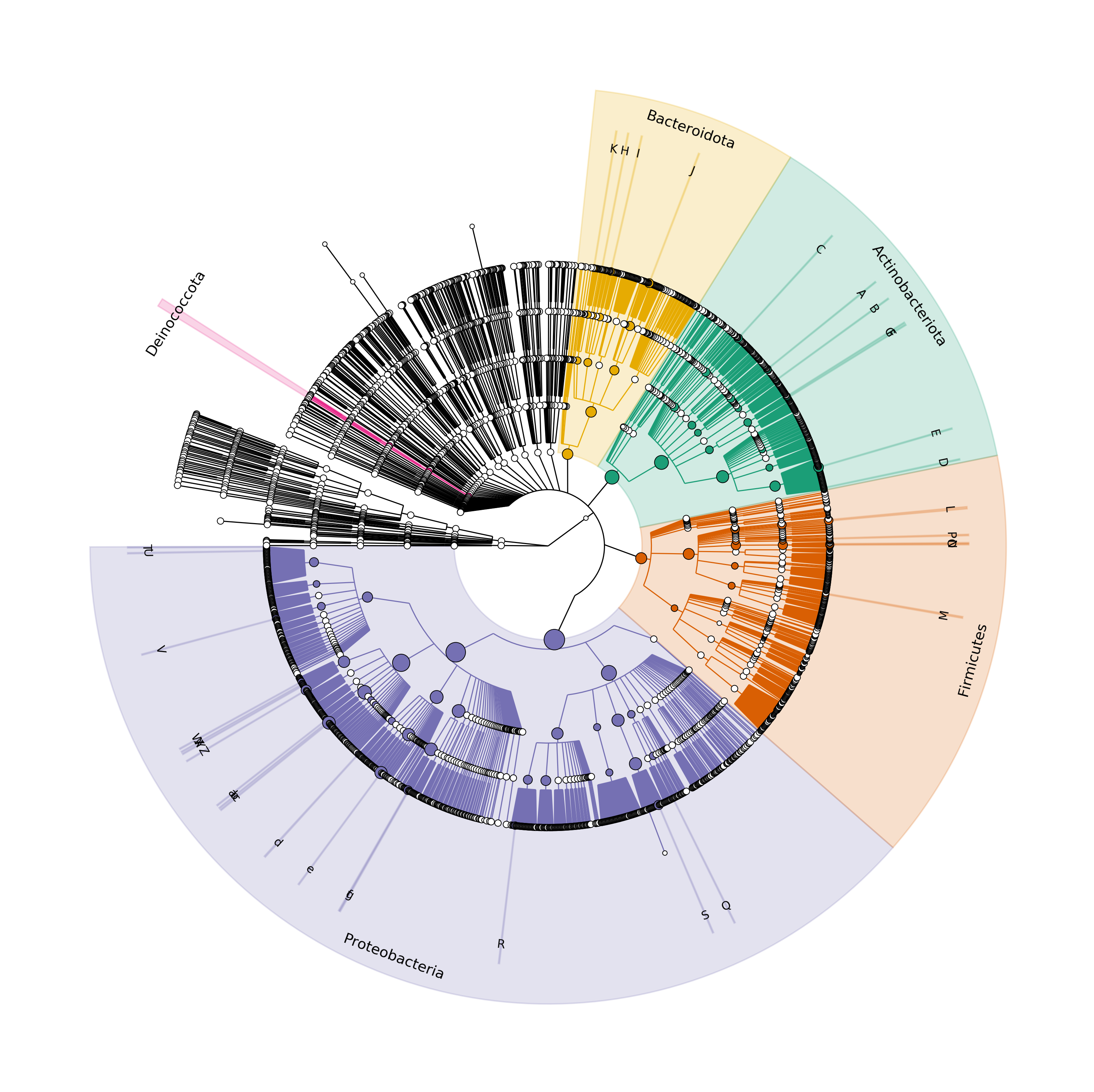
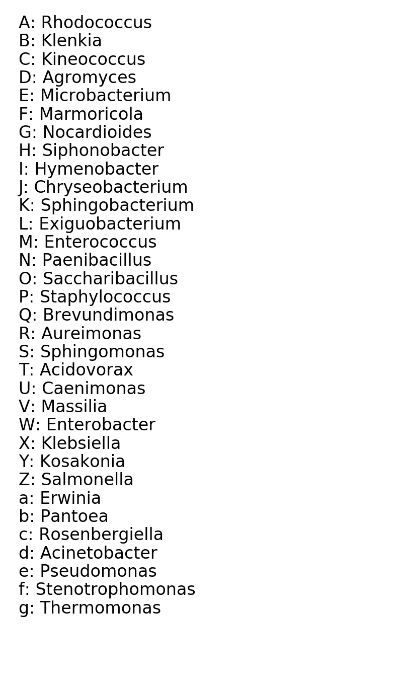
I will use the script silva-grafla.sh to generate the figure of the silva database.
$ sh silva-grafla.sh
Output files saved inside grap-files folder
Color for Bacteroidetes changed from 02d19ff to 0e6ab02
Color for Actinobacteria changed from 029cc36 to 0e7298a
Color for Firmicutes changed from 0ff3333 to 0d95f03
Color for Cyanobacteria changed from 000bfff to 01b9e77
Color for Bacteroidetes changed from 000ff80 to 07570b3
Generating the .png file
Finally, we obtained the desired image:

I will do the same for Greengenes and RDP databases with their own
scripts, green-grafla.sh and rdp-grafla.sh.
Here is the comparative of the three generated dendograms:
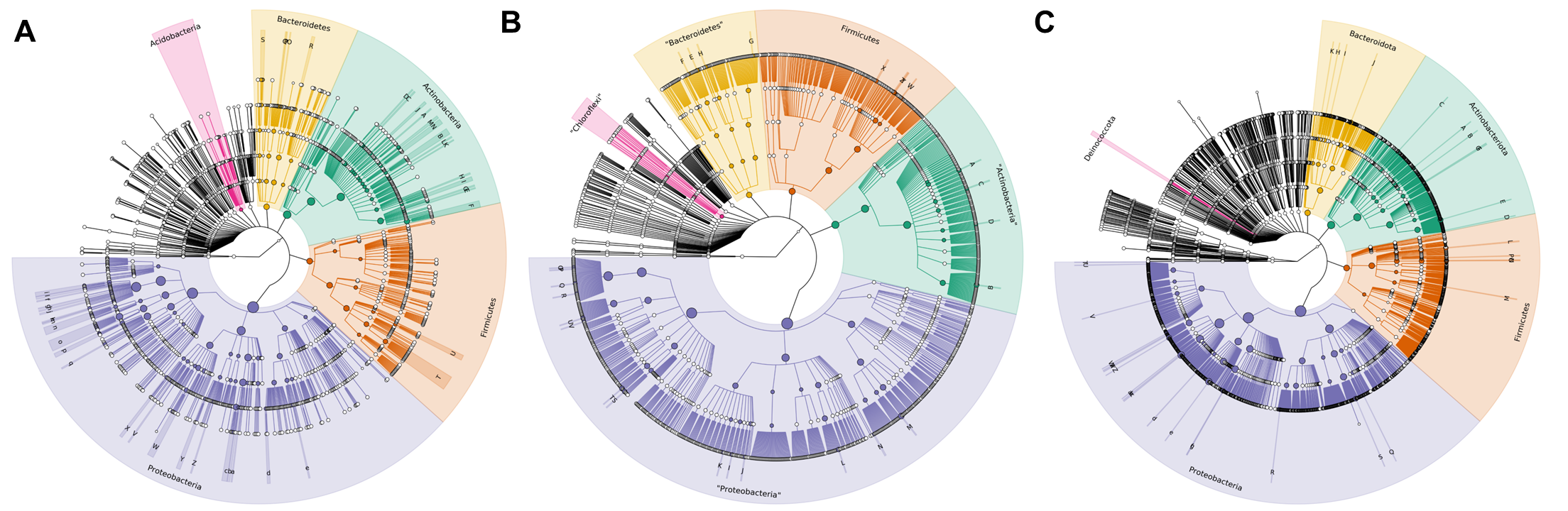
With this results, I conclude that the best database to work with will be
Greengenes.