clavibacter
Taxonomic exploration with R

First steps on exploring the data
![]()
Correction of kraken2 report output
In the last chapter, we processed all the data from Capsicum. I processed all the
Tuberosum libraries as well in order to have two sets of data from two
different host-plants to compare. First, I want to repeat that we are interested
in the different populations of Clavibacter species that are present in the
holobiont (plant). If we take a look in how kraken2 assignated the names of the
Clavibacter OTUs, we will see that we need to do some data trimming before we
can continue:
$ grep 'Clavibacter' capsicum/choi-2020/taxonomy/kraken/reports/SRR12778013.report
  0.00  544     84      G       1573                    Clavibacter
  0.00  398     151     S       28447                     Clavibacter michiganensis
  0.00  62      62      S1      1874630                     Clavibacter michiganensis subsp. capsici
  0.00  49      49      S1      31965                       Clavibacter michiganensis subsp. tessellarius
  0.00  33      33      S1      31964                       Clavibacter michiganensis subsp. sepedonicus
  0.00  32      32      S1      31963                       Clavibacter michiganensis subsp. nebraskensis
  0.00  29      29      S1      1401995                     Clavibacter michiganensis subsp. californiensis
  0.00  25      25      S1      33014                       Clavibacter michiganensis subsp. insidiosus
  0.00  17      15      S1      33013                       Clavibacter michiganensis subsp. michiganensis
  0.00  2       2       S2      443906                        Clavibacter michiganensis subsp. michiganensis NCPPB 382
  0.00  34      34      S       2768071                   Clavibacter zhangzhiyongii
  0.00  28      0       G1      2626594                   unclassified Clavibacter
  0.00  28      28      S       2860285                     Clavibacter sp. A6099
If we take a look to the information regarding this output, we can see that most of the
Clavibacter species that we are interested on, are clasiffied as subspecies of
Clavibacter michiganensis (e.g capsici, and tessellarius). I have created
a program that will correct this issue. The trim-clavi-reports.sh program is located
inside the scripts-folder
$ cat trim-clavi-reports.sh
#!/bin/bash

#This program is to trim the Clavibacter michiganensis identifiers from a kraken.report
#file

#The program will ask you 1 thing. a) The name of the report file

repo=$1 #Name of the report file
sufx=$(echo $repo |cut -d'.' -f1)

#Creating output directory
mkdir -p trim-reports


#Obtaining the values before Cmm
sed -n '/Clavibacter michiganensis/q;p' $repo > before-$sufx.txt

#Obtaining the C. michiganensis values
cat $repo | grep  'Clavibacter michiganensis' > cm-$sufx.txt

#Obtaining the values after Cmm
sed -n '/Clavibacter michiganensis/,$p' $repo | grep -v 'Clavibacter michiganensis'> after-$sufx.txt

# Taking the value of C. michiganensis
val1=$(grep 'michiganensis' cm-$sufx.txt | grep -v 'S2' | sed -n '1p' | cut  -f2)

#Obtaining the value that need to be substracted to the C. michiganensis field
i=0
grep 'michiganensis' cm-$sufx.txt | grep -v 'S2' | sed -n '1!p' | while read line;
do cou=$(echo $line | cut -d' ' -f2); i=$(($i + $cou)); echo $i ; done > temp
val2=$(tail -n1 temp)

##The new value
val3=$(($val1 - $val2))

#Making the new file of Clavi

##The first line with the unclassified Cm
a=$(grep 'michiganensis' cm-$sufx.txt | grep -v 'S2' | sed -n '1p' | cut  -f1)
b=$(grep 'michiganensis' cm-$sufx.txt | grep -v 'S2' | sed -n '1p' | cut  -f3)
c=$(grep 'michiganensis' cm-$sufx.txt | grep -v 'S2' | sed -n '1p' | cut  -f4)
d=$(grep 'michiganensis' cm-$sufx.txt | grep -v 'S2' | sed -n '1p' | cut  -f5)
e=$(grep 'michiganensis' cm-$sufx.txt | grep -v 'S2' | sed -n '1p' | cut  -f6)
echo " "$a"\t"$val3"\t"$b"\t"$c"\t"$d"\t""                  ""unclassified"$e > clavi.txt

##The rest of the species
grep 'michiganensis' cm-$sufx.txt | grep -v 'S2' | sed -n '1!p' | while read line;
do ta=$(echo $line | cut -d' ' -f1); tb=$(echo $line | cut -d' ' -f2);
tc=$(echo $line | cut -d' ' -f3); td=$(echo $line | cut -d' ' -f4);
te=$(echo $line | cut -d' ' -f5); tf=$(echo $line | cut -d' ' -f6);
tg=$(echo $line | cut -d' ' -f9);
echo "  "$ta"\t"$tb"\t"$tc"\t""S""\t"$te"\t""                  "$tf" "$tg >> clavi.txt ;
done

##The last line of the sub-sub species of Cmm
ka=$(grep 'michiganensis' cm-$sufx.txt | tail -n1| cut  -f1)
kb=$(grep 'michiganensis' cm-$sufx.txt | tail -n1| cut  -f2)
kc=$(grep 'michiganensis' cm-$sufx.txt | tail -n1| cut  -f3)
#kd
ke=$(grep 'michiganensis' cm-$sufx.txt | tail -n1| cut  -f5)
kf=$(grep 'michiganensis' cm-$sufx.txt | tail -n1| cut  -f6)
echo " "$ka"\t"$kb"\t"$kc"\t""S1""\t"$ke"\t""                   "$kf >> clavi.txt

#Creating the trimmed report
cat before-$sufx.txt > t-$sufx.report
cat clavi.txt >> t-$sufx.report
cat after-$sufx.txt >> t-$sufx.report

#Moving the new report to trim-reports
mv t-$sufx.report trim-reports/

#Removing temporary files
rm temp
rm cm-$sufx.txt
rm after-$sufx.txt
rm before-$sufx.txt
rm clavi.txt
Inside each of the reports folder, I will use the next line to run the program on all the outputs:
$ ls *.report | while read line; do sh parche.sh $line; done
Using kraken-biom to process the reports files
I will use kraken-biom to process all the reports and put them into a biom file. I will do an example inside the
capsicum/choi-2020/ folder:
$ mkdir biom-files/
$ kraken-biom reports/* --fmt json -o biom-files/choi-2020.biom
We will repear the same process for all the rest of the author’s folders.
Adjusting the all-aroun program
We will add this last step to the script that we have been constructing. We will
the user for a new input: 3) the name of a prefix, in this case the name of the
author. And we will get a new output inside the biom-files/ folder. The
kraken-biom.sh script inside the scripts folder
$ cat kraken-biom.sh
#!/bin/sh
# This is a program that is going to pick a SraRunTable of metadata and
#extract the run label to download, trim and move the libraries information.

# This program requires that you give 2 input data: 1) where this
#SraRunTable is located, and 2) where the kraken database has been saved

#ASSIGNATIONS
metd=$1 #Location to the SraRunTable.txt
kdat=$2 #Location of the kraken2 database
aut=$3 #A prefix to name some of the files. In this case, the author name.


root=$(pwd) #Gets the path to the directory of this file, on which the outputs ought to be created
# Now we will define were the reads are:
runs='reads'

# CREATING NECCESARY FOLDERS
mkdir reads
mkdir -p taxonomy/kraken
mkdir -p taxonomy/taxonomy-logs/scripts
mkdir -p taxonomy/kraken/reports
mkdir -p taxonomy/kraken/krakens
mkdir -p taxonomy/biom-files

# DOWNLOADING THE DATA

#Let's use the next piece of code to download the data
cat $metd  |  sed -n '1!p' | while read line;  do read=$(echo $line | cut -d',' -f1); fasterq-dump -S $read -p -e 8 -o $read ; done
mv *.fastq reads/
# The -e flag can be customized. This indicates the number of threads used to do this task.

# MANAGING THE DOWNLADED DATA

# We will change the names of the reads files. They have a sufix that makes impossible
#to be read in a loop
ls $runs | while read line ; do new=$(echo $line | sed 's/_/-/g'); mv $runs/$line $runs/$new; done

# Now, we will create a file where the information of the run labes can be located
cat $metd  | sed -n '1!p' | while read line; do read=$(echo $line | cut -d',' -f1); echo $read ; done > run-labels.txt
mv run-labels.txt metadata/

# TAXONOMIC ASSIGNATION WITH KRAKEN2

cat metadata/run-labels.txt | while read line; do file1=$(echo $runs/$line-1.fastq); file2=$(echo $runs/$line-2.fastq) ; echo '\n''working in run' "$line"\
#kraken2 --db $kdat --threads 6 --paired $file1 $file2 --output taxonomy/kraken/krakens/$line.kraken --report taxonomy/kraken/reports/$line.report \
echo '#!/bin/sh''\n''\n'"kraken2 --db $kdat --threads 6 --paired" "$runs/$line"'-1.fastq' "$runs/$line"'-2.fastq' "--output taxonomy/kraken/krakens/$line.kraken --report taxonomy/kraken/reports/$line.report" > taxonomy/taxonomy-logs/scripts/$line-kraken.sh; sh taxonomy/taxonomy-logs/scripts/$line-kraken.sh; done

#CREATING THE BIOM FILE

# Now we will create the biom file using kraken-biom
kraken-biom taxonomy/kraken/reports/* --fmt json -o taxonomy/biom-files/$aut.biom
Now, we will obtain the biom-file for all the author’s libraries in the next
time we run the script for the other host plants.
Note that in order to use the kraken-biom program, one needs ot install it. I install it in a conda environment
Using R for the analysis
Loading the packages
We will use a big set of packages for the analysis of the data. The main one
is phyloseq. We will load inside our
R environmnet the next set of packages:
> library("phyloseq")
> library("ggplot2")
> library("edgeR")
> library("DESeq2")
> library("RColorBrewer")
> library("stringr")
> library("sf")
> library("rnaturalearth")
> library("rnaturalearthdata")
> library("ggspatial")
> library("ggrepel")
> library("grid")
> library("gridExtra")
> library("ggmap")
> library("cowplot")
> library("ggsn")
> library("scatterpie")
Remember that some warnings can appear in the Console but do not be afraid. This
warnings are not errors that will preclude our management of the data.
Creating reliable palettes of colors
Since we will be managing different OTUs and we want to contrast the abundance of each ones, we will create two color palettes that will help us to have a diverse set of colors, all of them contrasting between each other.
The first one we will call it manual.colors
> manual.colors <- c('black','forestgreen', 'red2', 'orange', 'cornflowerblue',
                 'magenta', 'darkolivegreen4', 'indianred1', 'tan4', 'darkblue',
                 'mediumorchid1','firebrick4',  'yellowgreen', 'lightsalmon', 'tan3',
                 "tan1", 'wheat4', '#DDAD4B', 'chartreuse',
                 'seagreen1', 'moccasin', 'mediumvioletred', 'seagreen','cadetblue1',
                 "darkolivegreen1" ,"tan2" ,   "tomato3" , "#7CE3D8")
A second one, that will be useful for othe categorizations will be named
diverse.colors:
diverse.colors <- c("#1b9e77","#d95f02","#7570b3","#e7298a",
                    "#66a61e","#e6ab02","#a6761d","#666666")
Loading the biom files
We will load all the obtained biom files for the four folders, 3 from Capsicum, and 1 from Tuberosum:
> #Capsicum
> c.choi <- import_biom("../capsicum/choi-2020/taxonomy/biom-files/choi-2020.biom")
> c.misce <- import_biom("../capsicum/miscelaneous-capsicum/taxonomy/biom-files/miscelaneous-capsicum.biom")
> c.new <- import_biom("../capsicum/newberry-2020/taxonomy/biom-files/newberry-2020.biom")

#Tuberosum
> t.shi <- import_biom("../tuberosum/shi-2019/taxonomy/biom-files/shi-2019.biom")
We now have 4 new objects, each of them is a phyloseq object that has the
information of all the samples (libraries) of each author:
> c.choi
phyloseq-class experiment-level object
otu_table()   OTU Table:         [ 13193 taxa and 12 samples ]
sample_data() Sample Data:       [ 12 samples by 8 sample variables ]
tax_table()   Taxonomy Table:    [ 13193 taxa by 7 taxonomic ranks ]
Adjusting the biom data
We will use the next lines to trim the tax_table of each of the phyloseq
objects. We need to change the name of the columns to be meaningul, trim each of the names of the OTUs, and trim the names of the sample since the
kraken-biom.sh added a “t-“ before each name:
> #Capsicum
> c.choi@tax_table@.Data <- substring(c.choi@tax_table@.Data, 4)
> colnames(c.choi@tax_table@.Data) <- c("Kingdom", "Phylum", "Class", "Order", "Family", "Genus", "Species")
> colnames(c.choi@otu_table@.Data) <- substring(colnames(c.choi@otu_table@.Data), 3)

> c.misce@tax_table@.Data <- substring(c.misce@tax_table@.Data, 4)
> colnames(c.misce@tax_table@.Data) <- c("Kingdom", "Phylum", "Class", "Order", "Family", "Genus", "Species")
> colnames(c.misce@otu_table@.Data) <- substring(colnames(c.misce@otu_table@.Data), 3)

> c.new@tax_table@.Data <- substring(c.new@tax_table@.Data, 4)
colnames(c.new@tax_table@.Data) <- c("Kingdom", "Phylum", "Class", "Order", "Family", "Genus", "Species")
> colnames(c.new@otu_table@.Data) <- substring(colnames(c.new@otu_table@.Data), 3)

> #Tuberosum
> t.shi@tax_table@.Data <- substring(t.shi@tax_table@.Data, 4)
colnames(t.shi@tax_table@.Data) <- c("Kingdom", "Phylum", "Class", "Order", "Family", "Genus", "Species")
> colnames(t.shi@otu_table@.Data) <- substring(colnames(t.shi@otu_table@.Data), 3)
Loading and trimming the metadata
We already have the metadata of each set of data inside the metadata/ folder
in the SraRunTable.txt. We will use the next set of commands to load this
information to RStudio. Please note that I am leaving out one library
from the Capsucum/Newberry-2020 data (SRR10527395) and two libraries from
Tuberosum/Newberry-2020 (SRR7448326,SRR7457712) because the reads are in a
incompatibl format:
> #Capsicum
> ##Metadata from Capsicum/Choi-2020
> mraw.choi <- read.csv2(file = "../capsicum/choi-2020/metadata/SraRunTable.txt", sep = ",")
> ##Metadata from Capsicum/Miscelaneous
mraw.misce <- read.csv2(file = "../capsicum/miscelaneous-capsicum/metadata/SraRunTable.txt", sep = ",")
> ##Metadata from Capsicum/Newberry-2020
> mraw.new <- read.csv2(file = "../capsicum/newberry-2020/metadata/SraRunTable.txt", sep = ",")
> mraw.new <- mraw.new[! mraw.new$Run %in% c("SRR10527395"),]

> #Tuberosum
> ##Metadata from Tuberosum/Newberry-2020
> mraw.shi <- read.csv2(file = "../tuberosum/shi-2019/metadata/SraRunTable.txt", sep = ",")
> mraw.shi <- mraw.shi[! mraw.shi$Run %in% c("SRR7448326","SRR7457712"),]
But if we explore the metadata, we will see that there is a lot of information. Some of that information we do not need it and some need to be trimmed to use it. We will stablish the same structure for each metadata. This will include the next fields (Columns in the data.frame):
- Sample: Name of the sample.
- Plant: The host-plant of the sample
- Environment: Environmental circunstances where the plant was sampled
- Isolation: Part of the plant where the microbiome was sampled
- State: Disease or Healthy, I will use the letters D and H.
- Latitude: Coordinates where the sample was taken.
- Longitude: Coordinates where the sample was taken.
> ## Trimming the metadata
> #Capsicum
> met.choi <- data.frame(row.names = mraw.choi$Run,
                       Plant = rep("Capsicum", times = 12),
                       Sample= mraw.choi$Run,
                       Environment = rep("Field", times = 12),
                       Isolation= c(rep("Stem",4),rep("Root",4),rep("Stem",2),rep("Root",2)) ,
                       State= c("D","H","H","H","D","D","D","H","D","D","H","H"),
                       Latitude = rep(x = 25.811389, times = 12),
                       Longitude = rep(x= 106.523333, times = 12 ))
> met.misce <- data.frame(row.names = mraw.misce$Run,
                        Plant = rep("Capsicum", times = 4),
                        Sample = mraw.misce$Run,
                        Environment = c("Field","Field","Greenhouse","Field"),
                        Isolation = c(rep("Na", times = 4)),
                        State = c(rep("Na", times = 4)),
                        Latitude = c(rep("37.470000", times = 3),mraw.misce$geographic_location_.latitude.[4]),
                        Longitude = c(rep("127.970000", times = 3),mraw.misce$geographic_location_.longitude.[4]))
> met.new <- data.frame(row.names = mraw.new$Run,
                      Plant = rep("Capsicum", times = 3),
                      Sample = mraw.new$Run,
                      Environment = mraw.new$env_local_scale,
                      Isolation = mraw.new$env_medium,
                      State = rep("Na", times = length(mraw.new$Run)),
                      Latitude = c("32.601389","32.601389","33.20654") ,
                      Longitude = c("85.353611","85.353611","87.534607"))

> #Tuberosum
> met.shi <- data.frame(row.names = mraw.shi$Run,
                      Plant = rep("Tuberosum", times = 18),
                      Sample = mraw.shi$Run,
                      Environment = rep("Field", times = 18),
                      Isolation = rep("Soil", times = 18),
                      State = rep("D", times = 18),
                      Latitude = rep("34.2487", times = 18),
                      Longitude = rep("119.8167", times = 18))
Merging the information into new objects
First, we need to add the metadata of each set of samples to its corresponding
phyloseq object:
> #Capsicum
> c.choi <- merge_phyloseq(c.choi, sample_data(met.choi))
> c.misce <- merge_phyloseq(c.misce,sample_data(met.misce))
> c.new <- merge_phyloseq(c.new,sample_data(met.new))
> ##Merging all the three individual object in one that contains all the Capsicum data
> capsi <- merge_phyloseq(c.choi, c.misce, c.new)

> #Tuberosum
> tuber <- merge_phyloseq(t.shi, sample_data(met.shi))
Next, we will put all this together into the cbact phyloseq object, and all the
metadata into the all.meta object:
> ##Merging all 4 complete objects in one
> cbact <- merge_phyloseq(capsi,tuber)
> ##Concentrating the metadata in one object
> all.meta<- rbind(met.choi, met.misce, met.new, met.shi)
> cbact
phyloseq-class experiment-level object
otu_table()   OTU Table:         [ 14195 taxa and 37 samples ]
sample_data() Sample Data:       [ 37 samples by 8 sample variables ]
tax_table()   Taxonomy Table:    [ 14195 taxa by 7 taxonomic ranks ]
Normalization of the data
If we explore the depth of the different data that we have, we will see that is different between every sample. Since we will begin to plot the data, we will define the a vector containing the colors assigned to each plant, thus we will have a constant color pattern for the plant factor in each of the plots:
# We will create a vector to allocate the colors for each of the host plants that we have
plant.colors <- diverse.colors[1:length(unique(all.meta$Plant))]
names(plant.colors) <- unique(all.meta$Plant)
We also are going to create a folder to locate the figures we will be generating:
> dir.create("figures")
Now, we can create a figure to see the difference in the depth of the data:
> #Allocating the taxonomic information into a data.frame
> dprof <- data.frame(Samples = colnames(cbact@otu_table@.Data),
                    Reads = sample_sums(cbact),
                    Plant = cbact@sam_data@.Data[[2]])
> #Plotting the obtained data
> ggplot(data = dprof, mapping = aes(x = Samples, y = Reads))+
  geom_bar(stat = "identity", aes( fill = Plant)) +
  scale_fill_manual(values = c("cyan3","#EBA937"))+
  theme(text = element_text(size = 25),
        axis.text.x = element_text(angle = 90, hjust = 1, vjust = 0.5))
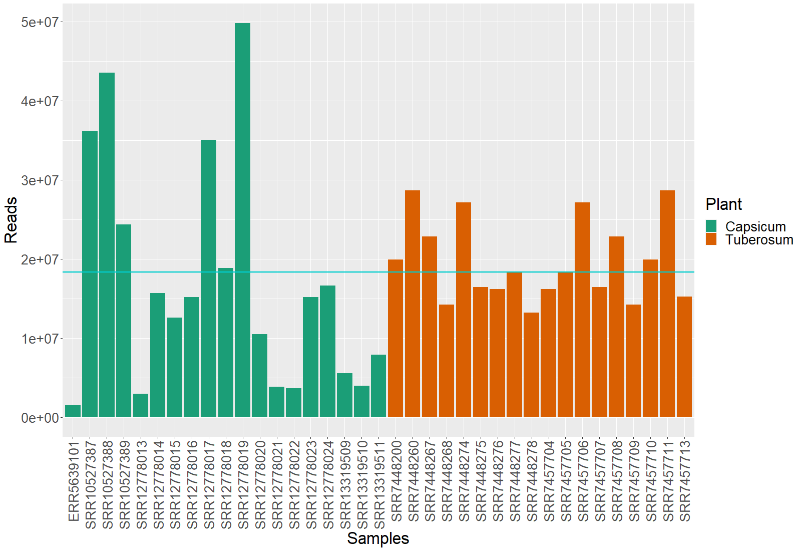
The cyan line marks the mean of the samples depth.
This makes is clear that the data needs normalization. McMurdi et al. found a great methodology to normalize the data. In their paper Waste Not, Want Not: Why Rarefying Microbiome Data Is Inadmissible they make an interesting discusion regarding this constant issue in this type of analysis. We will use their methodology:
> #-- Defining the normalization method --#
> edgeRnorm = function(physeq, ...) {
  require("edgeR")
  require("phyloseq")
  # physeq = simlist[['55000_1e-04']] z0 = simlisttmm[['55000_1e-04']] physeq
  # = simlist[['1000_0.2']] z0 = simlisttmm[['1000_0.2']] Enforce orientation.
  if (!taxa_are_rows(physeq)) {
    physeq <- t(physeq)
  }
  x = as(otu_table(physeq), "matrix")
  # See if adding a single observation, 1, everywhere (so not zeros) prevents
  # errors without needing to borrow and modify calcNormFactors (and its
  # dependent functions) It did. This fixed all problems.  Can the 1 be
  # reduced to something smaller and still work?
  x = x + 1
  # Now turn into a DGEList
  y = edgeR::DGEList(counts = x, remove.zeros = TRUE)
  # Perform edgeR-encoded normalization, using the specified method (...)
  z = edgeR::calcNormFactors(y, ...)
  # A check that we didn't divide by zero inside `calcNormFactors`
  if (!all(is.finite(z$samples$norm.factors))) {
    stop("Something wrong with edgeR::calcNormFactors on this data, non-finite $norm.factors")
  }
  # Don't need the following additional steps, which are also built-in to some
  # of the downstream distance methods. z1 = estimateCommonDisp(z) z2 =
  # estimateTagwiseDisp(z1)
  return(z)
}
> z<- edgeRnorm(cbact, method = "TMM")
> #-- Merging all the objects in the new normalized phyloseq object --#
> nor.cb <- merge_phyloseq(otu_table(z@.Data[[1]], taxa_are_rows = TRUE),
                         tax_table(cbact@tax_table@.Data),
                         cbact@sam_data)
> #Removing the dispensable created object
> rm(z)
Obtaining the Clavibacter data only
Since the scope of this work is to find the diversity of the Clavibacter
lineajes, we will extract this information from the data and put it in a new
object call clabac
> clabac <- subset_taxa(nor.cb, Genus == "Clavibacter")
> clavi.df <- psmelt(clabac)
> clavi.df$Species[clavi.df$Species==""] <- "sp."
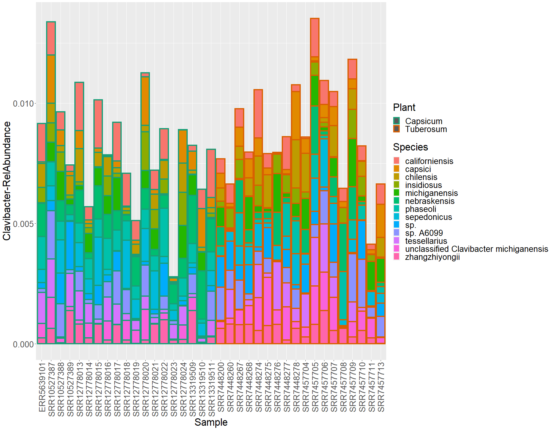
We will transform the abundance this to relative abundance to compare all the libraries between each other and plot the data:
# Transformation to relative abundance
clavi.df$ClaRelative <- sample_sums(clabac)/sample_sums(cbact)
#Plotting this data
ggplot(data = clavi.df, mapping = aes(y= ClaRelative, x = Sample, fill = Species, color = Plant))+
  geom_bar(position = "stack", stat = "identity", size=1.5)+
  scale_color_manual(values = plant.colors)+
  ylab(label = "Clavibacter-RelAbundance")+
  theme(text = element_text(size= 25),
        axis.text.x = element_text(angle = 90, hjust = 1, vjust = 0.5))
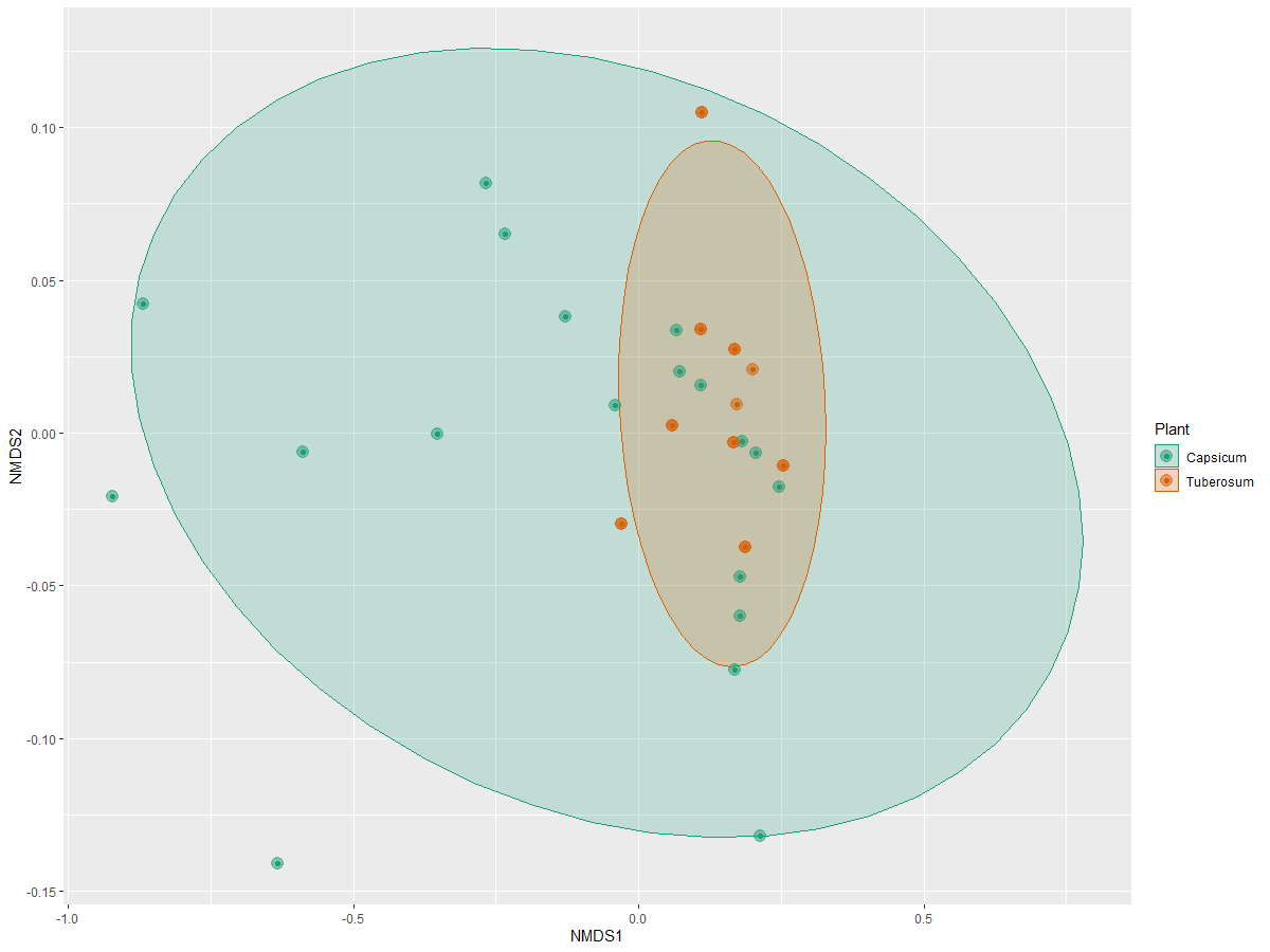
Now we will see what about the beta-diversity of this clavibacter data. First, we
will ordinate de data with phyloseq functions and we will plot it:
> clav.ord <- ordinate(physeq = clabac, method = "NMDS", distance = "bray")
> plot_ordination(physeq = clabac, ordination = clav.ord,
                color = "Plant") +
  stat_ellipse(geom = "polygon", alpha = 0.2, aes(fill = Plant))+
  geom_point(size=4 , alpha = 0.5)+
  scale_fill_manual(values = plant.colors)+
  scale_color_manual(values = plant.colors)
Preparing the data for plotting
Before we began, we need to coerce the Latitude and Longitude data from
characters to numeric data
> ## Coercing the coordinates to numeric
> all.meta$Latitude <- as.numeric(all.meta$Latitude)
> all.meta$Longitude <- as.numeric(all.meta$Longitude)
> # Also for clavi.df
> clavi.df$Latitude <- as.numeric(clavi.df$Latitude)
> clavi.df$Longitude <- as.numeric(clavi.df$Longitude)
We will create a new data.frame where we will locate the amplitude in coordinates
that we need to plot the data. This will be the maximum and minimum value of all
the sample’s Longitude and Latitude plus 2 and 1 respectively:
> ## Extracting the max and min value for all samples with a margin to allow the visualization of the data
> samp.sites <- data.frame(longitude= c(min(all.meta$Longitude)-2,max(all.meta$Longitude)+2),
                         latitude = c(min(all.meta$Latitude)-1,max(all.meta$Latitude)+1))
We will do a list where we will put all the information from just one sample in
each of its subsection. This subsection will have a new column to allocate the
Genus and Species information together:
> a <- list() # An empty list
> b <- NULL # An empty vector to locate the different Genus+Species diversity
> for (i in 1:length(unique(clavi.df$Sample))) {
    #Obtaining the data to work with inside a list
    a[[i]] <- clavi.df[clavi.df$Sample==unique(clavi.df$Sample)[i],]
    # Pasting the name of the Genus and Species in one new column
    a[[i]]$OTUName <- paste(a[[i]]$Genus, a[[i]]$Species, sep = "-")
    # We will define a vector to allocate all the different OTUs in case that not all the samples have the same ones
    b <- c(b,unique(a[[i]]$OTUName))
> }
> rm(i)
We will also stablis a vector to link each OTU name with a color from our
manual.colors vector:
> #We will take colors from the manual.colors vector as many unique OTUs in our data
> samp.colors <- rev(manual.colors)[1:(length(unique(b)))]
> # We will name this colors with the names of the unique OTUs
> names(samp.colors) <- unique(b)
We will use the scatterpie package to plot pie-graphs in the map. To accomplish this, we need a data frame that contains:
- Sample name
- Longitude
- Latitude
- Host plant
And a new column for each OTU present in all the samples that we want to graph, in this case, we need 13 columns.
Let’s get the Sample name Longitude,Latitude, and plant-hots information
> scatter.samples <- unique(clavi.df$Sample)
> scatter.Longitude <- NULL
> scatter.Latitude <- NULL
> scatter.Plant <- NULL
> for (i in 1:length(unique(clavi.df$Sample))) {
    scatter.Longitude[i] <- a[[i]]$Longitude[1]
    scatter.Latitude[i] <- a[[i]]$Latitude[1]
    scatter.Plant[i] <- a[[i]]$Plant[1]
> }
> rm(i)
> #Let's put the 4 vector into a data.frame
> scatter.data <- data.frame(scatter.samples, scatter.Longitude,scatter.Latitude, scatter.Plant)
> colnames(scatter.data) <- c("Sample","Longitude","Latitude","Plant")
Then, we need to put all the abundances of the different OTUs in a new data.frame
> # I will create an empty data.frame
> OTU.scatter <- data.frame(matrix(ncol = length(unique(b)),
                                   nrow = length(unique(clavi.df$Sample))))
> colnames(OTU.scatter) <- unique(b)
And fill this data.frame with the abundance information:
> for (i in 1:length(unique(b))) {
    O.Name <- NULL #Vector to put the abundance information of each OTU
    for (j in 1:length(unique(clavi.df$Sample))) {
      O.Name <- c(O.Name,a[[j]]$ClaRelative[a[[j]]$OTUName==unique(b)[i]])
    }
    OTU.scatter[i] <- O.Name #Filling each column
> }
> rm(i,j,O.Name,scatter.samples,
     scatter.Plant,scatter.Longitude,scatter.Latitude)
Finally, we will bind the two data.frames:
> scatter.data <- cbind(scatter.data,OTU.scatter)
> rm(OTU.scatter)
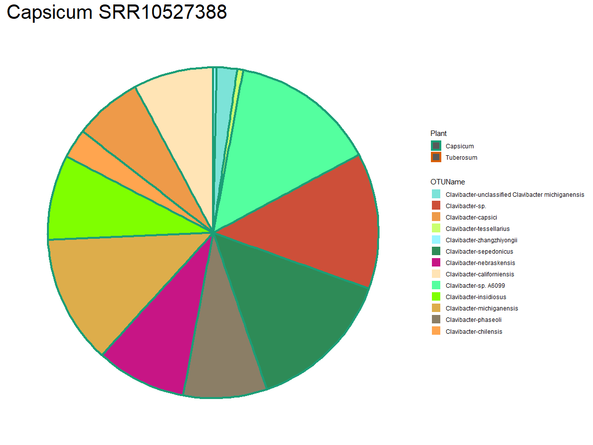
Plotting the data on a map and pie-graphs
We have all the information we need to generate the plots. First, we will create individual pie-graphs.
As an example, we will plot the first sample on our “a” list
> ggplot(data = a[[1]], mapping = aes(x = Sample, y = ClaRelative, fill= OTUName, color = Plant))+
    geom_bar(stat = "identity", width = 1, size= 1.5) +
    theme_bw()+
    scale_fill_manual(values = samp.colors) +
    scale_color_manual(values = plant.colors) +
    coord_polar("y", start=0)+
    ggtitle(paste(unique(a[[1]]$Plant),unique(a[[1]]$Sample), sep = " "))+
    theme(plot.title = element_text(size = 30),
          axis.line = element_blank(),
          axis.text.x = element_blank(),
          axis.text.y = element_blank(),
          axis.title.x = element_blank(),
          axis.title.y = element_blank(),
          axis.ticks=element_blank(),
          panel.background=element_blank(),
          panel.border=element_blank(),
          panel.grid.major=element_blank(),
          panel.grid.minor=element_blank(),
          plot.background=element_blank())
We will get this plots for all the samples and save them inside a new set of directories
> # Creating the folders that will contain the plots
> dir.create("pies/")
> dir.create("pies/labeled/")
> dir.create("pies/just-pie")
First, we will create the labeled pie graphs with the next for cycle and save
them inside the pies/labeled/ directory:
> l.pies <- list()
> for (i in 1:length(unique(clavi.df$Sample))) {
    l.pies[[i]] <- ggplot(data = a[[i]], mapping = aes(x = Sample, y = Abundance, fill= OTUName,color = Plant))+
      geom_bar(stat = "identity", width = 1,size= 0.6) +
      theme_bw()+
      scale_fill_manual(values = samp.colors) +
      scale_color_manual(values = plant.colors) +
      coord_polar("y", start=0)+
      ggtitle(paste(unique(a[[i]]$Plant),unique(a[[i]]$Sample), sep = " "))+
      theme(plot.title = element_text(size = 20),
            axis.line = element_blank(),
            axis.text.x = element_blank(),
            axis.text.y = element_blank(),
            axis.title.x = element_blank(),
            axis.title.y = element_blank(),
            axis.ticks=element_blank(),
            panel.background=element_blank(),
            panel.border=element_blank(),
            panel.grid.major=element_blank(),
            panel.grid.minor=element_blank(),
            plot.background=element_blank())
    ggsave(filename = paste(unique(clavi.df$Sample)[i],"png",sep = "."),dpi = 600,
           path = "pies/labeled/", width = 30, height = 20, units = "cm")
> }
> rm(i)
Now, we can do the ones without labels. Making them useful for diverse purposes:
> n.pies <- list()
> for (i in 1:length(unique(clavi.df$Sample))) {
    n.pies[[i]] <- ggplot(data = a[[i]], mapping = aes(x = Sample, y = Abundance, fill= OTUName,color = Plant))+
      geom_bar(stat = "identity", width = 1,size= 0.6) +
      theme_bw()+
      scale_fill_manual(values = samp.colors) +
      scale_color_manual(values = plant.colors) +
      coord_polar("y", start=0)+
      theme(axis.line = element_blank(),
            axis.text.x = element_blank(),
            axis.text.y = element_blank(),
            axis.title.x = element_blank(),
            axis.title.y = element_blank(),
            axis.ticks=element_blank(),
            panel.background=element_blank(),
            panel.border=element_blank(),
            panel.grid.major=element_blank(),
            panel.grid.minor=element_blank(),
            plot.background=element_blank(),
            legend.position="none")
    ggsave(filename = paste(unique(clavi.df$Sample)[i],"png",sep = "."),dpi = 600,
           path = "pies/just-pie/", width = 20, height = 20, units = "cm")
> }
> rm(i)
Let’s put this pie-graphs over the map.
We will use the map_data function to load the information we need.
> mi.world <- map_data(map = "world")
Then we will use the geom_polygon function from ggplot2 to plot the map. We will
use the coord_fixed option to delimit the map to the coordinate range from the
samples:
> ggplot(mi.world, mapping = aes(x = long, y = lat, group = group))+
    geom_polygon(fill= "gray",colour = "black")+
    xlab("Longitude") + ylab("Latitude") + theme_bw()+
    coord_fixed(xlim = samp.sites$longitude,
                ylim = samp.sites$latitude,
                expand = TRUE)
> ggsave(filename = paste("03-05-nakedMap","png",sep = "."),dpi = 900,
         path = "figures/", width = 30, height = 20, units = "cm")
Finally, we will use the geom_scatterpie from the scatterpie package to put
the pies over this map:
> ggplot(mi.world, mapping = aes(x = long, y = lat, group = group))+
    geom_polygon(fill= "gray",colour = "black")+
    xlab("Longitude") + ylab("Latitude") + theme_bw()+
    coord_fixed(xlim = samp.sites$longitude,
                ylim = samp.sites$latitude,
                expand = TRUE) +
    geom_scatterpie(data = scatter.data, cols = unique(b),
                    pie_scale = 0.6,
                    aes(x= Longitude , y = Latitude, color = Plant))+
    scale_fill_manual(values = samp.colors) +
    scale_color_manual(aesthetics = c("color"),values = plant.colors)
  ggsave(filename = paste("03-06-MapWPies","png",sep = "."),dpi = 1200,
         path = "figures/", width = 30, height = 15, units = "cm")
As you can see, there is still an issue with this plot because we have more than one sample with the same coordinates and the pie-charts overlap.