From-kraken-to-graphlan

From kraken to graphlan

I got enthralled by figures representing metagenomic taxonomic assignation and phylogenies using graphlan. During my master’s degree research project, I tried different taxonomic assignation programs (one of them was MetaPhlAn), but the one that gave me the best results was kraken. After reading a little bit and trying to find a way to traduce my kraken output to work with graphlan I found a way to generate this good-looking figures using the kraken output. In order to obtain this desired results we will use the next set of softwares:

Software	Version	Manual
kraken2	2.1.2	Link
krakentools	1.2	Link
graphlan	1.1.3	Link
export2graphlan	0.22	Link

Recommended Setup

#Make sure that your python version is compatible with export2graphlan.py script, in my case I created an enviroment with python2.7 #conda create –name py27 python=2.7 #Activate the enviroment when using export2graphlan conda activate py27

Taxonomic assignation with kraken2

A team from I am part of have develop a lesson on The Carpentries platform where the taxonomic assingnation is explained. Here, I will leave an example code only for ilustrative purpose, but I will like to highlight that in order to use kraken2 for taxonomic assignation, a machine (or cluster) with at least 64 Gb of RAM, 200 Gb of disk space, and 12 cores is recommended:

mkdir taxonomy/kraken

kraken2 --db kraken-db --threads 12 --paired --fastq-input $file1 $file2 --output taxonomy/kraken/prefix_kraken.kraken --report taxonomy/kraken/prefix_kraken.report
bracken -d kraken-db -i taxonomy/kraken/prefix_kraken.report -o taxonomy/kraken/prefix.bracken

Where the file1 and file2 are the files where the forward and reverse reads are resepctively localized, and the prefix a disired identification that you want to give to all your working files from that sample.

In order to follow the next steps without requiring to download the reads files, I attached the resulting kraken2 reports from a set of samples from the work Population genomics of cycad coralloid-root bacterial microbiome in contrasting environments(Unpublished) to serve as an example of the following steps.

The kraken reports for this example are located in the reports folder in the GitHub-page

Using krakentools

Lets put everything in a folder that we will call kraken-to-graphlan inside any locality of your computer. Inside this folder we will create a folder to relocate the .report files, we will call it kraken-reports. Move the reports to this new folder to end with a folder-structure as follows:

As part of the tools offered by krakentools, there is a function called kreport2mpa.py. This program takes the kraken2 output report file and generate a MetaPhlAn-style text file that we will use.

$ tree

.
└── kraken-reports
    ├── QroArlegundo_kraken.report
    ├── QroDCuatro_kraken.report
    ├── QroPocitos1_kraken.report
    ├── QroPocitos2_kraken.report
    ├── SLPCarrizal1_kraken.report
    ├── SLPCarrizal2_kraken.report
    └── SLPLimones_kraken.report

If we call the the kreport2mpa.py in the terminal, we will obtain an output explaining the way to use it:

kreport2mpa.py

usage: kreport2mpa.py [-h] -r R_FILE -o O_FILE [--display-header]
                      [--read_count] [--percentages] [--intermediate-ranks]
                      [--no-intermediate-ranks]
kreport2mpa.py: error: the following arguments are required: -r/--report-file/--report, -o/--output

You can use this program to process each report separately. We will take the report QroPocitos1_kraken.report to explain this by using the next piece of code:

$ kreport2mpa.py -r kraken-reports/QroPocitos1_kraken.report -o QroPocitos1.mpa
$ ls

QroPocitos1.mpa  kraken-reports

If we explore the insides of this new file, we will obtained a MetaPhlan-style text file:

$ head -n 10 QroPocitos1.mpa

k__Bacteria     11123979
k__Bacteria|p__Cyanobacteria    10675084
k__Bacteria|p__Cyanobacteria|o__Nostocales      10608906
k__Bacteria|p__Cyanobacteria|o__Nostocales|f__Nostocaceae       9978629
k__Bacteria|p__Cyanobacteria|o__Nostocales|f__Nostocaceae|g__Nostoc     9834713
k__Bacteria|p__Cyanobacteria|o__Nostocales|f__Nostocaceae|g__Nostoc|s__Nostoc_sp._'Lobaria_pulmonaria_(5183)_cyanobiont'      4719169
k__Bacteria|p__Cyanobacteria|o__Nostocales|f__Nostocaceae|g__Nostoc|s__Nostoc_flagelliforme     1144071
k__Bacteria|p__Cyanobacteria|o__Nostocales|f__Nostocaceae|g__Nostoc|s__Nostoc_linckia   956414
k__Bacteria|p__Cyanobacteria|o__Nostocales|f__Nostocaceae|g__Nostoc|s__Nostoc_punctiforme       916756k__Bacteria|p__Cyanobacteria|o__Nostocales|f__Nostocaceae|g__Nostoc|s__Nostoc_sp._'Peltigera_membranacea_cyanobiont'_N6       801547

To maintain a good organization of this little example, let’s create a folder where we will locate the mpa files and move this output there.

$ mkdir mpa-files
$ mv QroPocitos1.mpa mpa-files/

For different reasons, is desireable to process a group of report files together to display the taxonomic assignation of a set of samples. We will do this with all the report files we have in our kraken-reports folder using the next piece of code:

$ ls kraken-reports/*.report | while read line; do name=$(echo $line | cut -d'/' -f2 |cut -d'_' -f1); kreport2mpa.py -r $line -o mpa-files/$name.mpa; done

And we will combine this .mpa files into one with the program combine_mpa.py. To use it, we will need to specify the .mpa files that we want to combine and the name of the output file:

$ combine_mpa.py --input mpa-files/*.mpa --output mpa-files/combine.mpa

 Number of files to parse: 7
 Number of classifications to write: 5495
        5495 classifications printed

$ ls mpa-files/

QroArlegundo.mpa  QroPocitos1.mpa  SLPCarrizal1.mpa  SLPLimones.mpa
QroDCuatro.mpa    QroPocitos2.mpa  SLPCarrizal2.mpa  combine.mpa

By exploring the new file, we will se that we have all the samples integrated in columns in this new .mpa file:

$ head -n10 combine.mpa

#Classification Sample #1       Sample #2       Sample #3       Sample #4       Sample #5       Sample #6       Sample #7
k__Bacteria     13023490        15523665        11123979        5990058 9812341 13672293        13687393
k__Bacteria|p__Coprothermobacterota     0       1       3       2       2       2       0
k__Bacteria|p__Coprothermobacterota|c__Coprothermobacteria      0       1       3       2       2       2       0
k__Bacteria|p__Coprothermobacterota|c__Coprothermobacteria|o__Coprothermobacterales     0       1       3       2       2       2       0
k__Bacteria|p__Coprothermobacterota|c__Coprothermobacteria|o__Coprothermobacterales|f__Coprothermobacteraceae   0       1       3       2       2       2       0
k__Bacteria|p__Coprothermobacterota|c__Coprothermobacteria|o__Coprothermobacterales|f__Coprothermobacteraceae|g__Coprothermobacter      0       1       3       2       2       2       0
k__Bacteria|p__Coprothermobacterota|c__Coprothermobacteria|o__Coprothermobacterales|f__Coprothermobacteraceae|g__Coprothermobacter|s__Coprothermobacter_proteolyticus   0       1       3       2       2       0
k__Bacteria|p__Chrysiogenetes   5       10      18      79      0       237     4
k__Bacteria|p__Chrysiogenetes|c__Chrysiogenetes 5       10      18      79      0       237     4

Adjusting Cyanobacterial OTUs

If we pay close inspection to how Cyanobacteria are classified, we will see something unexpected. We will se that the majority of the Cyanobacterial OTUs do not have an assigned Class to its classification.

$ grep "Cyanobacteria" combine.mpa | head -n 10

k__Bacteria|p__Cyanobacteria    11970156        15042312        10675084        5286452 9045418 13337317       11338702
k__Bacteria|p__Cyanobacteria|o__Gloeoemargaritales      57      23      9       535     265     24    8
k__Bacteria|p__Cyanobacteria|o__Gloeoemargaritales|f__Gloeomargaritaceae        57      23      9     535      265     24      8
k__Bacteria|p__Cyanobacteria|o__Gloeoemargaritales|f__Gloeomargaritaceae|g__Gloeomargarita      57    23       9       535     265     24      8
k__Bacteria|p__Cyanobacteria|o__Gloeoemargaritales|f__Gloeomargaritaceae|g__Gloeomargarita|s__Gloeomargarita_lithophora        57      23      9       535     265     24      8
k__Bacteria|p__Cyanobacteria|c__Gloeobacteria   290     2684    224     176     147     856     166
k__Bacteria|p__Cyanobacteria|c__Gloeobacteria|o__Gloeobacterales        290     2684    224     176   147      856     166
k__Bacteria|p__Cyanobacteria|c__Gloeobacteria|o__Gloeobacterales|f__Gloeobacteraceae    290     2684  224      176     147     856     166
k__Bacteria|p__Cyanobacteria|c__Gloeobacteria|o__Gloeobacterales|f__Gloeobacteraceae|g__Gloeobacter   290      2684    224     176     147     856     166
k__Bacteria|p__Cyanobacteria|c__Gloeobacteria|o__Gloeobacterales|f__Gloeobacteraceae|g__Gloeobacter|s__Gloeobacter_kilaueensis 6       15      53      9       4       834     154

This is a serious problem, because as we will see in the final graph, each of the taxonomic levels will be a node in the final dendogram. So, almost all Cyanobacteria will have a shorter arm that the rest of the OTUs. If for any reason you do not have the above problem (e.g kraken2 database version), you can continue to the next section ““

First, let’s see which of the Cyanobacterial OTUs have an assigned Class:

$ grep "Cyanobacteria" combine.mpa | grep c__

k__Bacteria|p__Cyanobacteria|c__Gloeobacteria   290     2684    224     176     147     856     166
k__Bacteria|p__Cyanobacteria|c__Gloeobacteria|o__Gloeobacterales        290     2684    224     176  147      856     166
k__Bacteria|p__Cyanobacteria|c__Gloeobacteria|o__Gloeobacterales|f__Gloeobacteraceae    290     2684 224      176     147     856     166
k__Bacteria|p__Cyanobacteria|c__Gloeobacteria|o__Gloeobacterales|f__Gloeobacteraceae|g__Gloeobacter  290      2684    224     176     147     856     166
k__Bacteria|p__Cyanobacteria|c__Gloeobacteria|o__Gloeobacterales|f__Gloeobacteraceae|g__Gloeobacter|s__Gloeobacter_kilaueensis        6       15      53      9       4       834     154
k__Bacteria|p__Cyanobacteria|c__Gloeobacteria|o__Gloeobacterales|f__Gloeobacteraceae|g__Gloeobacter|s__Gloeobacter_violaceus  284     2669    169     167     143     20      12

There are some OTUs with the Gloeobacteria Class assigned. So we will need to make some adjustments to the file. We will extract the number of reads assigned to the Gloeobacteria Class in the first sample with the next line of code

$ cat combine.mpa | grep Cyanobacteria | grep Gloeobacteria| sed -n '1p'| cut -f2

290

Let’s try to untangle the code a little bit. sed -n '1p' will help us to get just the first line of the result after searching for Gloeobacteria; cut -f2 will print the abundance of the first sample. Now, we will assign this value to a variable that we will call x1:

$ x1=$(cat combine.mpa | grep Cyanobacteria | grep Gloeobacteria| sed -n '1p'| cut -f2)
$ echo $x1

290

We will also need to obtain the value of the Cyanobacterial counts, so that we can supress the value of Gloeobacteria from the rest of the Cyanobacterial counts. Let’s do it for the first sample an assign the value to a variable y1:

$ y1=$(cat combine.mpa | grep Cyanobacteria |sed -n '1p'| cut -f2)
$ echo $y1

11970156

Finally, we will substract the x1 from the y1 value and store it in a new variable called z1:

$ z1=$(echo $(($y1 - $x1)))
$ echo $z1

11969866

As you can see in the structure of the file combine.mpa, each superior level of classification cotains all the abundance of the reads in its inferior OTUs. For example, the 57 reads of the species _Gloeomargarita_lithophora in sample one are contained in the total amount of reads of Cyanobacteria (i.e. 11970156) for that first sample:

$ grep "Cyanobacteria" combine.mpa | sed -n '5p'

k__Bacteria|p__Cyanobacteria|o__Gloeoemargaritales|f__Gloeomargaritaceae|g__Gloeomargarita|s__Gloeomargarita_lithophora        57      23      9       535     265     24      8

grep "Cyanobacteria" combine.mpa | sed -n '1p'

k__Bacteria|p__Cyanobacteria    11970156        15042312        10675084        5286452 9045418 13337317       11338702

That is why we need this substraction, we need to create a new line for the missing Class c__Cyanophyceae, which will contain all the reads assigned to the phylum cyanobacteria with the exception of those with the Gloeobacteria Class. So, we need to do this for each of the seven samples. Included in this repository there is the folder scripts where the scripts that we will use are located. Inside, you can find a file called cyano-operations.sh, move it to the mpa-files folder. We will use this script to trim our Cyanobacterial OTUs. I want to explain what some of this lines are going to do:

$ tail -n 18 cyano-operations.sh

# We will begin to assemble the cyano.mpa file, where the trimmed information will be allocated.
# Extract the p__Cyanobacteria first line of information ans put it in a new file
cat combine.mpa | grep Cyanobacteria | sed -n '1p'|head > cyanos.mpa
# Now we will add the Gloeobacteria lines
cat combine.mpa | grep Cyanobacteria | sed -n '1!p'| grep Gloeobacteria >> cyanos.mpa
# Then, we will create a line for the new class
cat combine.mpa | grep Cyanobacteria | sed -n '1p'| while read line; do first=$(echo $line | cut -d' ' -f1); second=$(echo $line | cut -d' ' -f2,3,4,5,6,7,8 ); echo $first"|c__Cyanophyceae\t"$z1"\t"$z2"\t"$z3"\t"$z4"\t"$z5"\t"$z6; done >> cyanos.mpa
# Moreover, add the rest of the lines with the next command:
cat combine.mpa | grep Cyanobacteria | sed -n '1!p'| grep -v Gloeobacteria| while read line; do first=$(echo $line | cut -d'|' -f1,2); second=$(echo $line | cut -d'|' -f3,4,5,6,7,8 ); echo $first"|c__Cyanophyceae|"$second; done >> cyanos.mpa

# We will use awk to create tab separations instead of blank spaces
awk -v OFS="\t" '$1=$1' cyanos.mpa > cyano.mpa
# Remove the old cyanos.mpa file
rm cyanos.mpa

#Let's add this trimmed information to the entire data
cat combine.mpa | grep  -v Cyanobacteria > trim-combine.mpa
cat cyano.mpa >> trim-combine.mpa

We will run the cyano-operations.sh and see that this will generate two new files cyano.mpa trim-combine.mpa:

$ sh cyano-operations.sh
$ ls

QroArlegundo.mpa  QroPocitos2.mpa   SLPLimones.mpa       cyano.mpa
QroDCuatro.mpa    SLPCarrizal1.mpa  combine.mpa          trim-combine.mpa
QroPocitos1.mpa   SLPCarrizal2.mpa  cyano-operations.sh

cyano.mpa is where the trimmed OTUs are saved, and trim-combine.mpa is the new .mpa object where this Cyanobacterial OTUs and the rest of them are combined. As you can see, now the Cyanobacterial OTUs have a Class assignet to them:

$ grep 'Cyanobacteria' trim-combine.mpa | grep -v 'c__Gloeobacteria'| head -n5

k__Bacteria|p__Cyanobacteria    11970156        15042312        10675084        5286452 9045418 13337317       11338702
k__Bacteria|p__Cyanobacteria|c__Cyanophyceae    11969866        15039628        10674860        5286279045271  13336461
k__Bacteria|p__Cyanobacteria|c__Cyanophyceae|o__Gloeoemargaritales      57      23      9       535   265      24      8
k__Bacteria|p__Cyanobacteria|c__Cyanophyceae|o__Gloeoemargaritales|f__Gloeomargaritaceae        57    23       9       535     265     24      8
k__Bacteria|p__Cyanobacteria|c__Cyanophyceae|o__Gloeoemargaritales|f__Gloeomargaritaceae|g__Gloeomargarita     57      23      9       535     265     24      8

Generate the plot

We will return to the above folder kraken-to-graphlan to proceed to the next step of this tutorial. In the scripts folder you will find a file named grafla.sh , download it inside your kraken-to-graphlan folder.

$ cat grafla.sh

#!/bin/sh

mkdir grap-files

export2graphlan.py --skip_rows 1,2 -i mpa-files/trim-combine.mpa --tree grap-files/merged_abundance.tree.txt \
--annotation grap-files/merged_abundance.annot.txt --most_abundant 100 --annotations 2 \
--external_annotations 6 --abundance_threshold 15 --ftop 1000 \
--annotation_legend_font_size 8 --def_font_size 30
echo Output files saved inside grap-files folder

echo Color for Bacteroidetes changed from $#2d19ff to $#e6ab02
sed 's/#2d19ff/#e6ab02/g' grap-files/merged_abundance.annot.txt > temp.txt && mv temp.txt grap-files/merged_abundance.annot.txt

echo Color for Actinobacteria changed from $#29cc36 to $#e7298a
sed 's/#29cc36/#e7298a/g' grap-files/merged_abundance.annot.txt > temp.txt && mv temp.txt grap-files/merged_abundance.annot.txt

echo Color for Firmicutes changed from $#ff3333 to $#d95f03
sed 's/#ff3333/#d95f03/g' grap-files/merged_abundance.annot.txt > temp.txt && mv temp.txt grap-files/merged_abundance.annot.txt

echo Color for Cyanobacteria changed from $#00bfff to $#1b9e77
sed 's/#00bfff/#1b9e77/g' grap-files/merged_abundance.annot.txt > temp.txt && mv temp.txt grap-files/merged_abundance.annot.txt

echo Color for Bacteroidetes changed from $#00ff80 to $#7570b3
sed 's/#00ff80/#7570b3/g' grap-files/merged_abundance.annot.txt > temp.txt && mv temp.txt grap-files/merged_abundance.annot.txt


graphlan_annotate.py --annot grap-files/merged_abundance.annot.txt grap-files/merged_abundance.tree.txt grap-files/merged_abundance.xml

echo Generating the .png file
graphlan.py --dpi 300 --size 10 grap-files/merged_abundance.xml graphlan_graph.png --external_legends

All the inital parameters from the export2graphlan.py can be found in its GitHub repository. This programm gives a predertermined set of colors to highlight the most abundant OTUs at different taxonomic level. This can be changed by different ways, but the option that I am showing here changes also the colors of all the highlighted OTUs inside the dominant Phyla. This changes must be done in the merged_abundance.annot.txt file. So the lines of code that beggin with the function sed, are changing the default colors. As posted in graphlan repository, the last four lines of code generate a .xml file that will dictate the instructions for graphlan.py to generate the cladogram graphlan_graph.png.

Let’s run it and see the new files that this will generate:

$ sh grafla.sh
$ ls

Now we have a nwe folder grap-files and three .png files. Inside graphlan_graph.png is the desired plot.

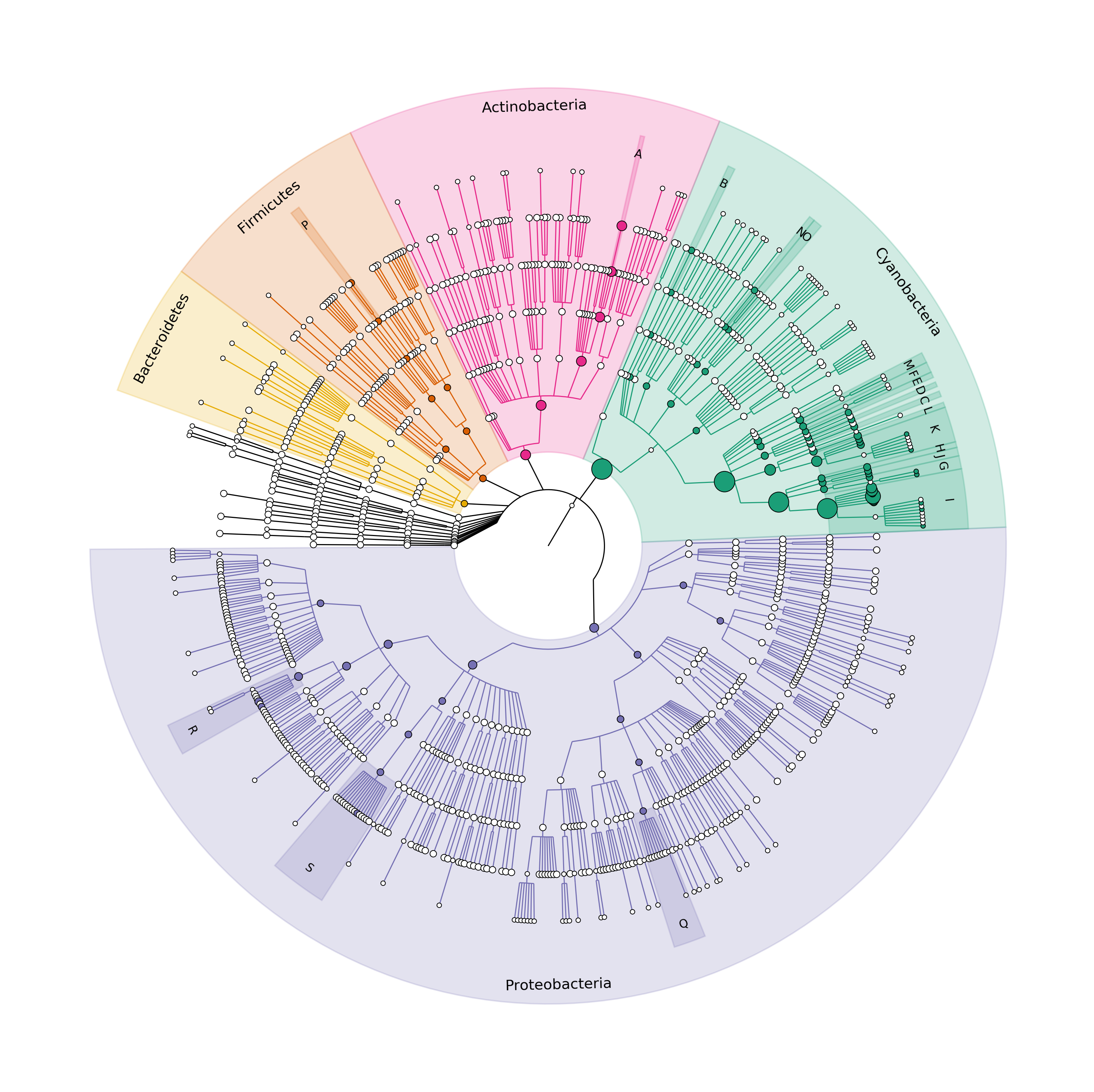
Figure 1. Cladogram where the dominant Phyla are highlighted and the dominant Genera as well.

Inside the other two .png files we will find the legend and annotation of the highlighted Phyla and Genera respectively. This is delivered in this way because we used the flag --external_legends for the graphlan.py program.

Figure 2. The legend of the dominant Phyla in the main plot.

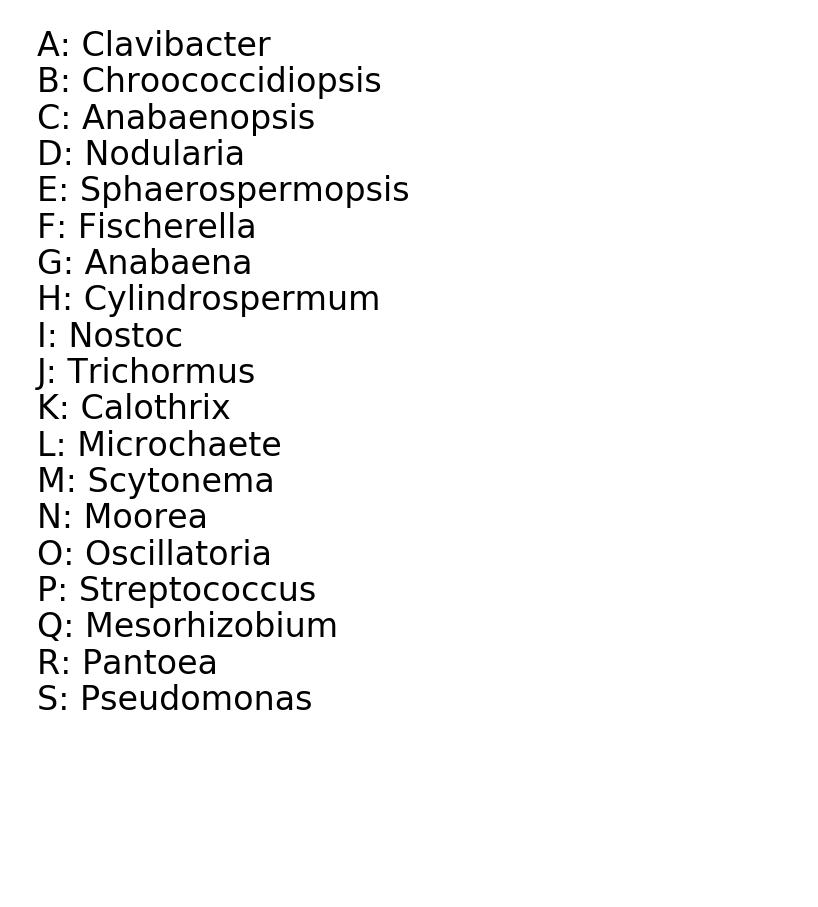
Figure 3. Annotation of the dominan Genera.

Adding rings to the figure

Right now, we have generated a good looking plot. But an astonishing trait of graphlan is the annotation rings that can be created around the cladogram. We will try to generate them with the existing data. Unfortunately, the manipulation of the characteristics of the final plot is not so intuitive…in a sense is like really crafting a piece of art. I will show you here the way the route that I used, but I imagine there are tons of them. Again, in the scripts folder you will find the need files for generating this rings. We will do it in three steps.

Assigning the ring information to all the Phyla and Genera

We will use the get-rings.sh script to generate the needed files to begin. Let’s see what it is inside this little script.

$ cat get-rings.sh

#!/bin/sh

mkdir rings-files

cat grap-files/merged_abundance.annot.txt | grep p__ | grep clade_marker_size \
| while read line; do otu=$(echo $line | cut -d' ' -f1) ; \
value=$(echo $line | cut -d' ' -f3); \
echo $otu"\tring_alpha\t"1"\t"$value;done > rings-files/ring1.txt
cat grap-files/merged_abundance.annot.txt | grep g__ | grep clade_marker_size \
| while read line; do otu=$(echo $line | cut -d' ' -f1) ; \
value=$(echo $line | cut -d' ' -f3); \
echo $otu"\tring_height\t"2"\t"$value;done > rings-files/ring2.txt

echo New files are locates in the rings-files folder

By running the little script, we will have a new set of files. ring1.txt and ring2.txt will have the information for the first and second ring respectively.

$ sh get-rings.sh
$ more rings-files/ring1.txt

p__Acidobacteria        ring_alpha      1       20.0321277763
p__Actinobacteria       ring_alpha      1       46.9110777016
p__Bacteroidetes        ring_alpha      1       20.5406403465
p__Chlorobi     ring_alpha      1       20.0145017817
p__Chloroflexi  ring_alpha      1       20.0164002978
p__Cyanobacteria        ring_alpha      1       200.0
p__Deinococcus_Thermus  ring_alpha      1       10.0
p__Firmicutes   ring_alpha      1       21.9076866623
p__Fusobacteria ring_alpha      1       20.0600717798
p__Gemmatimonadetes     ring_alpha      1       20.0127499699
p__Planctomycetes       ring_alpha      1       20.0800518513
p__Proteobacteria       ring_alpha      1       38.191719665
p__Spirochaetes ring_alpha      1       20.0572668289
p__Tenericutes  ring_alpha      1       20.0761845479
p__Thermotogae  ring_alpha      1       20.0108880536
p__Verrucomicrobia      ring_alpha      1       20.0197569815

If we inspect what is inside ring1.txt, we will see a tab separated file of 4 columns with the Phylum identification, the ring type, the ring number and the abundance value. As described in the graphlan repository, we need this this fourth column to have values between 0 and 1, we need to normalize the data.

Using R to normalize the data

Now, we will use the script named norm-rings.R script to normalize the data. First, we will change the working directory of our RStudio environment into the kraken-to-graphlan folder:

> setwd("~/kraken-to-graphlan")

Substitute the ~ symbol for the apropiate path to access this location. Next, wer will define a function to normalize the data.

> norm1 <- function(x){(x-min(x))/(max(x)-min(x))}

We will read the data from the file ring1.txt and use the defined function to change the data in the fourth column i.e. the abundance:

> ring1 <- read.table(file = "rings-files/ring1.txt")
> ring1$V4 <- norm1(ring1$V4)

Finally, let’s write a new object for where our normalized data will be lovated

> write.table(ring1, file = "rings-files/tring1.txt", sep ="\t" ,
            row.names = FALSE, col.names = FALSE, quote = FALSE)

We will do the same for the ring2.txt file:

> ring2 <- read.table(file = "rings-files/ring2.txt")
> ring2$V4 <- norm1(ring2$V4)
> write.table(ring2, file = "rings-files/tring2.txt", sep ="\t" ,
            row.names = FALSE, col.names = FALSE, quote = FALSE)

Add the information to the annotation file and remade the plot

For this last step, we will use two scripts: polish.rings.sh and final-grafla.sh.

Let’s see what it is inside polish.rings.sh:

$ cat polish.rings.sh

#!/bin/sh

cat grap-files/merged_abundance.annot.txt | grep p__ | grep clade_marker_size \
| while read line; do otu=$(echo $line | cut -d' ' -f1) ; \
value=$(echo $line | cut -d' ' -f3); \
echo $otu"\tring_color\t"1"\t#AAAA00";done >> rings-files/tring1.txt

cat rings-files/tring1.txt >> grap-files/merged_abundance.annot.txt
cat rings-files/tring2.txt >> grap-files/merged_abundance.annot.txt

echo color added to the first ring

echo -e "ring_label\t"1"\tPhyla-abundance" >> grap-files/merged_abundance.annot.txt
echo -e "ring_label\t"2"\tGenera-abundance" >> grap-files/merged_abundance.annot.txt

echo Label created for the two rings in the plot

The first line of code is very similar to what we saw inside the get-rings.sh script and is used to add the color #AAAA00 to the first ring. Then, all the information from tring1.txt and tring2.txt is concatenated inside merged_abundance.annot.txt, alongside the names for this two rings.

$ sh polish.rings.sh
$ more rings-files/tring1.txt

p__Acidobacteria        ring_alpha      1       0.0528006725068421
p__Actinobacteria       ring_alpha      1       0.194268830008421
p__Bacteroidetes        ring_alpha      1       0.0554770544552632
p__Chlorobi     ring_alpha      1       0.0527079041142105
p__Chloroflexi  ring_alpha      1       0.0527178963042105
p__Cyanobacteria        ring_alpha      1       1
p__Deinococcus_Thermus  ring_alpha      1       0
p__Firmicutes   ring_alpha      1       0.0626720350647369
p__Fusobacteria ring_alpha      1       0.0529477462094737
p__Gemmatimonadetes     ring_alpha      1       0.0526986840521053
p__Planctomycetes       ring_alpha      1       0.0530529044805263
p__Proteobacteria       ring_alpha      1       0.148377471921053
p__Spirochaetes ring_alpha      1       0.05293298331
p__Tenericutes  ring_alpha      1       0.0530325502521053
p__Thermotogae  ring_alpha      1       0.0526888844926316
p__Verrucomicrobia      ring_alpha      1       0.0527355630605263
p__Acidobacteria        ring_color      1       #AAAA00
p__Actinobacteria       ring_color      1       #AAAA00
p__Bacteroidetes        ring_color      1       #AAAA00
p__Chlorobi     ring_color      1       #AAAA00
p__Chloroflexi  ring_color      1       #AAAA00
p__Cyanobacteria        ring_color      1       #AAAA00
p__Deinococcus_Thermus  ring_color      1       #AAAA00
p__Firmicutes   ring_color      1       #AAAA00
p__Fusobacteria ring_color      1       #AAAA00
p__Gemmatimonadetes     ring_color      1       #AAAA00
p__Planctomycetes       ring_color      1       #AAAA00
p__Proteobacteria       ring_color      1       #AAAA00
p__Spirochaetes ring_color      1       #AAAA00
p__Tenericutes  ring_color      1       #AAAA00
p__Thermotogae  ring_color      1       #AAAA00
p__Verrucomicrobia      ring_color      1       #AAAA00

Finally, we will use final-grafla.sh to create the plot with the rings:

$ sh final-grafla.sh
$ ls *.png

final_graph.png        final_graph_legend.png  graphlan_graph_annot.png
final_graph_annot.png  graphlan_graph.png      graphlan_graph_legend.png

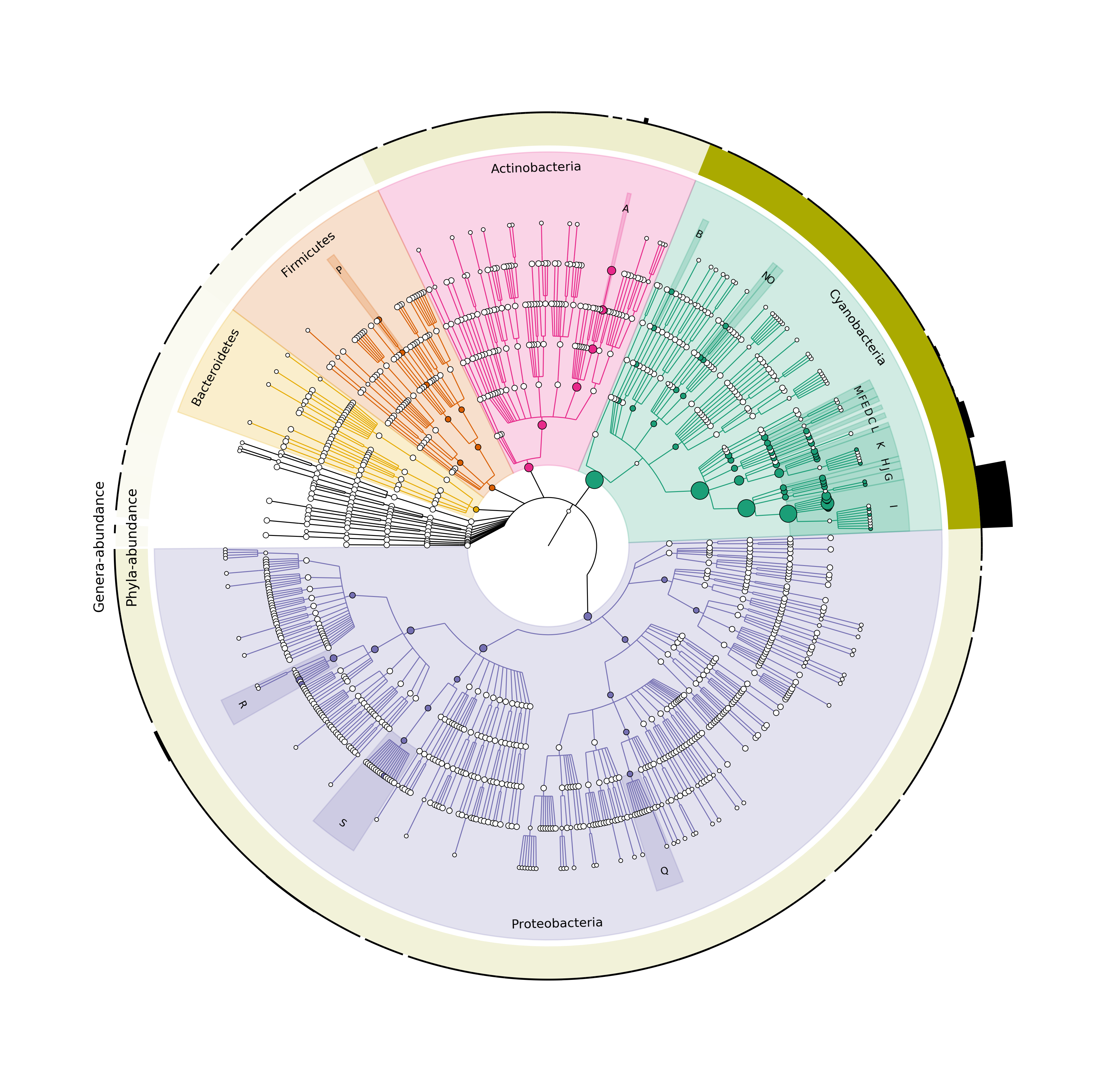
Figure 4. Final Cladogram with all the final adjustments.

This took me early-mornings and nights to grok. This is the main reason why I desired to share it not only by the code, but with an explanatory document to help other fellow bioinformatician to cope with the academic life.